This post is intended to start a discussion – and ideally identify what data might be available to address this problem further. The analysis presented is preliminary in nature, and could almost certainly be refined. I would really value a discussion of this with colleagues who read it.
Accident risk
In studies of road and rail vehicles in cross winds, some estimate of the risk of an accident is often required. If the critical accident wind speed for a particular vehicle is known, then my approach in the past has been to use the probability distribution for the hourly mean wind speed (assumed to be a Weibull distribution) and the probability distribution for the turbulence fluctuations around this average (assumed to be a normal distribution) to calculate the percentage of time that this critical value is exceeded, through a convolution of the two distributions. Additionally, when wind-warning systems are being developed, the question often arises as to what would be an appropriate mean wind speed at which to limit vehicle movements. This can be derived by calculating the percentage of time that the critical wind speed is exceeded from the probability distributions for turbulence fluctuations, for a range of mean wind speeds, and then choosing a value that has an acceptable level of risk.
In some recent work that I have carried out for a particular client, it has become clear to me that this approach is not really adequate – an example of practical reality not always conforming with attractive theoretical approaches! Both road and rail vehicles require a gust to be above the critical value for a specific period of timebefore an accident occurs. This period of time is usually between 0.5s and 3s, the time it takes for a vehicle to actually blow over. Thus in determining the risk of an accident what is really required is some idea of the number of times the critical wind speed is exceeded, N, for more than (say) T seconds for a particular mean wind speed U. This is not the same as the proportion of time for which the critical wind speed is exceeded, as some these exceedances will often last for less than T seconds. If the probability of N for any particular U is known, then this can be convoluted with the probability distribution for U to calculate the overall risk, or used to determine an appropriate value of U for wind warning systems.
To the best of my knowledge, the specification of the number of gusts N lasting greater than a specific time T for a particular mean wind speed has not been investigated in the past – but if any reader knows of such work, I would be glad to hear of it. In this post, I present the results of a preliminary investigation into this problem.
The data
In what follows, I will use two experimental wind datasets as follows.
- Data from that late 1990s obtained at the Wind Engineering field site at Silsoe Research Institute, and in particular two one-hour datasets (Silsoe 1 and Silsoe 2) with wind velocities measured at 10Hz at 3, 6 and 10m above the ground, for 10m wind speeds of 9.7 and 10.5m/s.
- Data from Storm Ophelia in 2017, obtained from measurements at the top of the Muirhead Tower at the University of Birmingham, 72m above the ground, measured at 10Hz, for mean hourly wind speeds of 10.4, 12.5 and 13.8m/s (Birmingham 1, Birmingham 2 and Birmingham 3). With thanks to Dr Mike Jesson of the University of Birmingham for making this data available
The basic statistics for each hour of data is given in table 1.

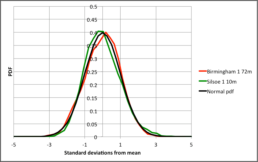
From this table it can be seen that the Silsoe site has a surface roughness length (determined from velocity profiles) typical of smooth rural environments (0.005m), with turbulence intensities (standard deviation / mean values) that are consistent with such an environment and which fall slightly with height. The Birmingham data was obtained at one point high above a suburban environments, and thus the surface roughness length cannot be determined from a velocity profile, but can be expected to be an order of magnitude or more higher than at the Silsoe site. The turbulence intensity is similar to that measured at Silsoe, although the measurements were made at a much greater height above the ground. For the Silsoe data the probability distributions of the data all show a positive skew, whilst the Birmingham data show both positive and negative skew values that are much closer to zero. Typical examples of such distributions are shown in figure 1. The Silsoe near-ground distribution has a significantly longer upper tail, than the Birmingham values high above the ground, i.e. a significant skew towards the higher velocities. This may well be because of individual sweep events in the atmospheric boundary layer being more significant near to ground level. The normal distribution, which I have assumed in the past for my calculations, does not fit either dataset particularly well.
Analysis of exceedances
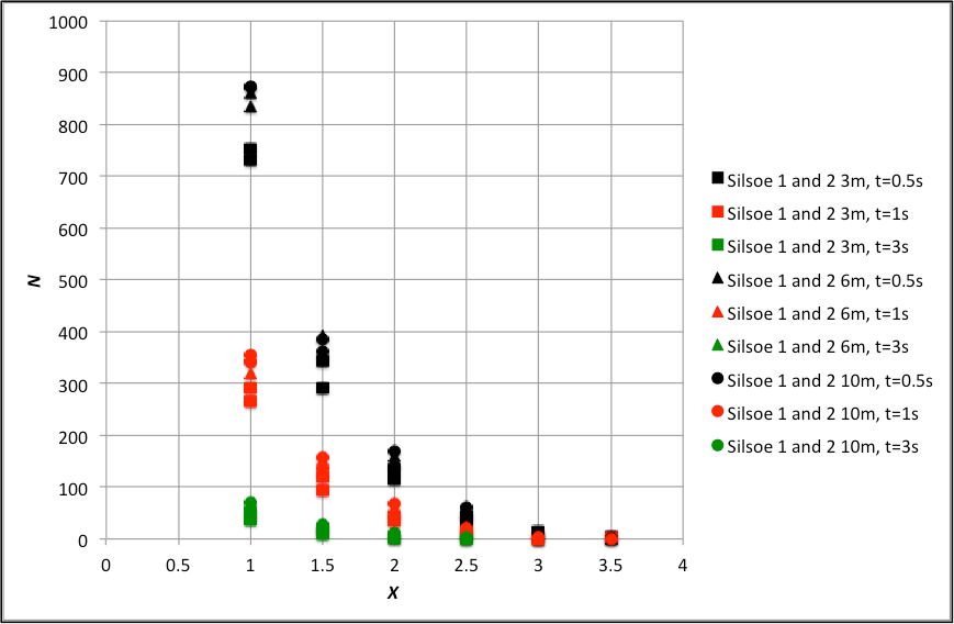
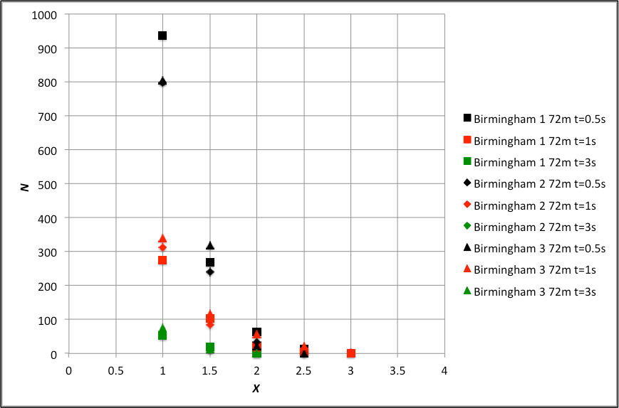
The approach to using this data has been to find, for each dataset, the number of exceedances N for T= 0.5s, 1s and 3s gusts above a range of velocity levels above the mean. To enable comparison between the different datasets, these velocities are expressed in terms of standard deviations above the mean, denoted by X. The results are shown in figure 2 for the Silsoe data and figure 3 for the University of Birmingham data. The following comments can be made.
- N falls as T increases, which is only to be expected.
- The value of X at which N falls to zero falls as T increases, as again is to be expected. This value is around 3 to 3.5 for the Silsoe data, and 2.5 to 3 for the Birmingham data, reflecting the form of the tail of the probability distributions discussed above.
- For the Silsoe data, the results for the two datasets are very similar and there is an indication that N varies with height above the ground.
- The Birmingham datasets also have similar results, and there is no discernable effect of wind speed in the data when plotted in this way.
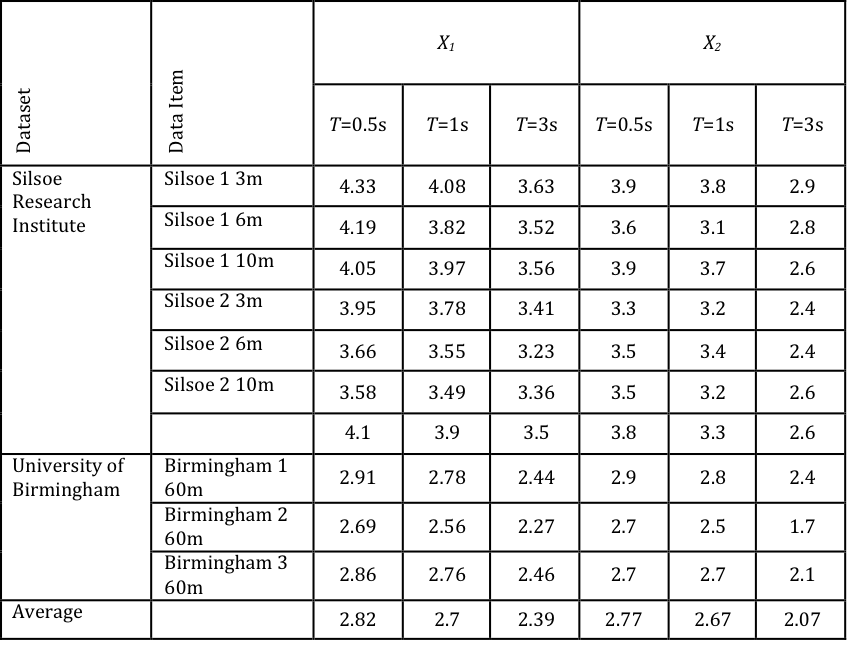
Clearly the distributions of N have an upper limit. This can be characterized in two ways.
- By the value of X for which the probability of the wind speed exceed T/3600, X1
- By the highest value of X for which N>0, X2
Both these values of X are shown in table 2 for the various datasets. It can be seen that there is some variability in the results, which is inevitable as we are dealing with the tails of the distribution where data becomes discontinuous. In general the values for X1 are higher than those for X2, particularly for the near ground Silsoe data, suggesting that the use of simple probabilities rather than gust numbers may well significantly overestimate vehicle overturning risk. Both values fall as the time period T increases as would be expected, and the values for the Silsoe data are significantly higher than for the Birmingham data, which again follows from the difference in probability distributions. The equivalent values for X1 for a normal probability distribution are 3.64, 3.45 and 3.14, for T= 0.5, 1 and 3s respectively. It can thus be seen from Table 2 that the Silsoe values lie above the normal distribution values, and the Birmingham values lie significantly below them.
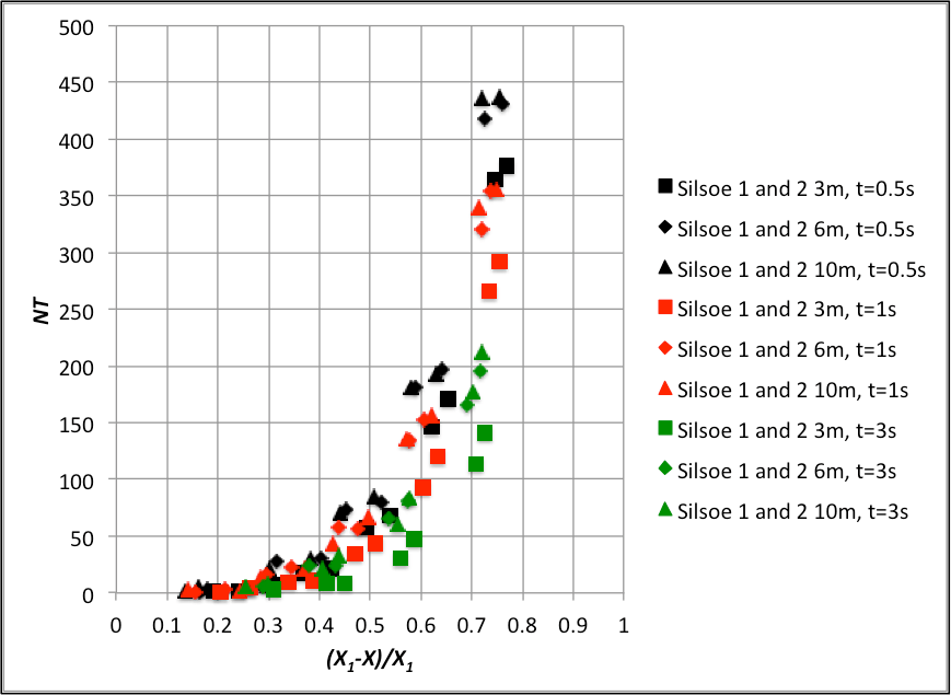
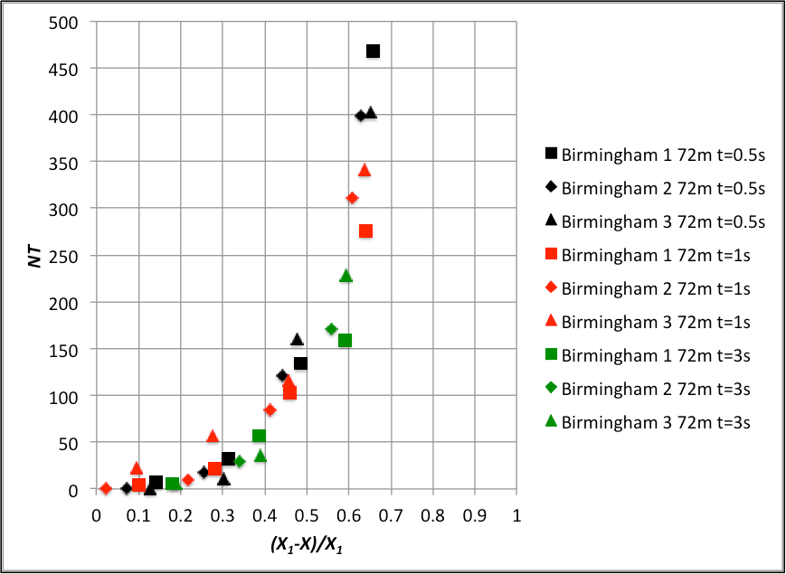
The data from figures 2 and 3 thus appears to be consistent and sensible, but the question then arises as to how this data can be parameterized to enable it to be used easily in calculations. After some trial and error analysis it was found that all the data for each site could be made to collapse around a single curve by plotting the combined variables NT and (X1-X)/X1 against each other. These variables seem sensible, as both are dimensionless, with the former giving a normalised value of number of exceedances, and the latter describing being the difference between specific gust velocities, and the value at which N must be zero. The results are shown in figures 4 and 5 for the Silsoe and Birmingham data respectively, using the measured values of X1 for each dataset. It can be seen there is much scatter, but the data collapse is reasonably good. The two sets of data do not however coincide, indicating the effects of the underlying shape of the probability distribution, and in particular the upper tails.
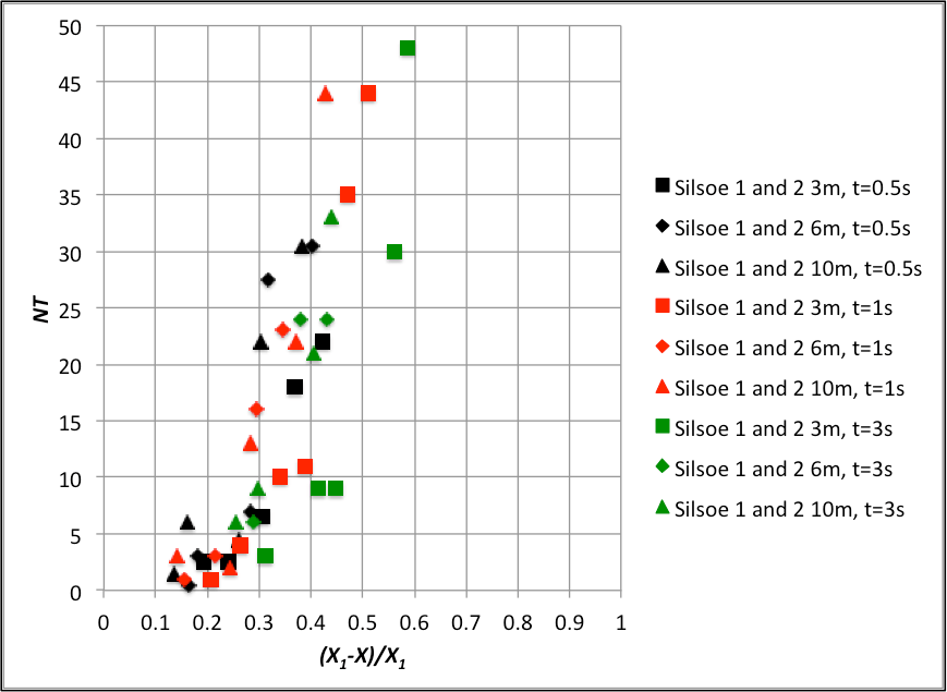
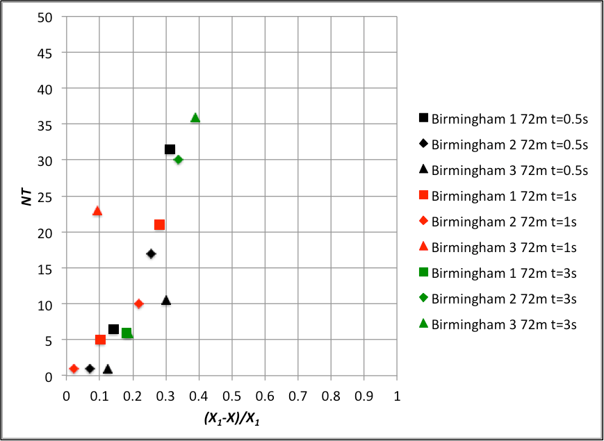
The region of most practical interest on these data collation is for a low number of events, since these represent conditions where the risk might be tolerable. Thus figures 6 and 7 thus show expanded versions of figures 4 and 5 for NT<50. It would quite possible to fit lines or curves to this data, although the best fit values would be different between the Birmingham and Silsoe datasets.
It would seem that if this method is to become useful in a predictive, rather more detailed information on near ground probability distributions is required for a variety of ground roughness conditions / heights above the ground etc., so that the variation in the exceedance curves of figures 4 to 7 can be more fully understood and an overall data collation be achieved. If any reader knows of systematic data for wind probability distributions, please let me know.
