Preamble
Most modern trains are “sealed” in that they are designed to minimise the leakage of air between the inside and the outside of the cabin. There are a number of reasons for this. Firstly HVAC systems require as little leakage as possible to be able to operate efficiently. Secondly, when a train passes through a tunnel at speed, it generates large pressure transients that can cause passenger aural discomfort and pain – sealing the train attenuates or even eliminates such transients in the train interior. However the sealing of trains is never perfect and some way of quantifying leakage is required, and then of calculating the internal pressure of trains for the types of external pressure field experienced as trains pass through tunnels, allowing for this leakage. This brief post looks at the standard methodology for doing this, which is essentially empirical, and compares it firstly with methods for the calculation of leakage in buildings used by ventilation engineers, which are based on the concept of an equivalent orifice, and secondly with a new method which models leakage paths as simple pipe flows. It is shown that the empirical model currently used is consistent with the new leakage pipe model, and the use of the latter enables some of the limitations of the current method to be more fully appreciated.
The railway methodology
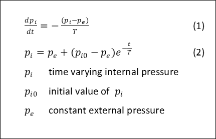
The standard method for assessing how well a train is sealed is to pump air into the train to raise the internal pressure to a specified level and then simply to observe the decay of pressure when the pump is turned off. It is then assumed that this pressure decay follows the simple rate equation shown in equation (1), which can be solved to give the exponential decay expression of equation (2) The parameter T is a leakage time constant and can usefully be used to quantify the degree of sealing (Note that this is usually denoted by the Greek letter tau, but this website is unable to cope with Greek letters in the text). Tests are usually carried out for static trains but can in principle be carried out for moving trains, where one might expect the degree of sealing to be somewhat less than the static case due to the relative movement of different parts of the train envelope. Thus two values of the leakage time are often defined – Tstatic and Tdynamic. The sealing criteria themselves vary somewhat around the world and are usually expressed in terms of a minimum time for the pressure to fall from one specified value to another. These criteria are usefully summarised in Niu et al (2020). The range of criteria effectively imply values of T of the order of 10 to 60 seconds. Once a value of T has been determined, equation (1) can be used in reverse to find how the internal pressure varies for rapidly varying external pressures, such as when trains pass through tunnels. This usually requires a numerical solution to equation (1).
The calculation of leakage in buildings
Now the approach taken in the study of building ventilation is somewhat different. A number of authors, for example Harris (1990) developed an equation for the flow in and out of buildings with both major openings such as windows, and with a distributed minor leakage openings. For the case of leakage only, which is most analogous to the train case, the basic expression used in given in equation (3). This is effectively an equation for flow through an orifice, and the basic assumption is that the leakage area can be represented by an equivalent orifice. It is then assumed that the change in internal pressure is an adiabatic process, and thus equation (4) applies. I am not altogether sure why the process should be adiabatic rather than isothermal, but that is probably due to my lack of understanding of thermodynamics. Putting these equations together gives equation (5), which is equivalent to equation (1) except that the change in internal pressure is proportional to the root of the difference between the external and internal pressures, rather than being directly proportional.

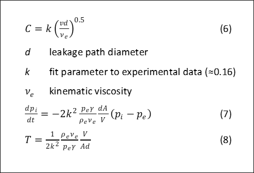
Now the analysis that leads to equation (5) assumes that the orifice coefficient remains constant. However, at low orifice Reynolds numbers, the coefficient is known to fall significantly – see Johansen (1930) and the figure below. (I find I have rather a perverse pleasure at quoting a technical paper that is almost 100 years old!). This implies that equation (5) can only be valid when the pressure differences, and associated leakage flow rates, are quite high. To investigate this further, on the basis of the experimental results shown in the figure below, we take the discharge coefficient to vary with the square root of the Reynolds number as in equation (6). Here the Reynolds number is based on the leakage velocity v and the average diameter of a single leakage path d (which can be expected to have a very much smaller area than the overall leakage area A). After some manipulation this results in equation (7). This is of exactly the same form as equation (1), and the leakage time constant can be explicitly expressed as in equation (8).

There is still however an issue in applying this equivalent orifice analysis to the case of train leakage. From equation (3) above, the velocity through the orifice is directly related to the pressure difference, with the energy loss being described by the discharge coefficient. For the values of pressure difference across building facades, which are of the order of tens of Pascals, typical values of the discharge coefficient of around 0.6, result in velocities through the orifice are of the order of 1m/s. The pressure differences between the inside and outside of trains in tunnels however can be up to 2 or 3Pa, and an orifice type analysis would give velocities of 40 or 50m/s, which is clearly unrealistic. The discharge coefficient method therefore does not give an adequate energy loss to the leakage flow for high pressure differentials. So this type of analysis may be applicable in building ventilation, but does not seem appropriate for the consideration of train leakage. Some other framework needs to be developed to give the railway methodology for calculating leakage something other than an empirical basis.
Leakage tube methodology
As an alternative, it is possible to conceive of the leakage paths on a train as a set of equivalent pipes. Equation (3) can then be written in the form of equation (9) – which is effectively Darcy’s law for flow through a pipe. The energy loss in the system is determined by the Darcy friction factor. After some manipulation one arrives at the expression of equation (10), which is equivalent to equation (5). Now for high Reynolds numbers (> around 2000) the Darcy friction factor will be constant, and the rate of change of pressure will be proportional to the root of the pressure difference between inside and outside the train – as in the orifice flow analysis. However at low Reynolds numbers the Darcy friction factor varies inversely with Reynolds number as shown. This results in equation (11), which gives the rate of change of internal pressure as being proportional to the difference between the external and internal pressures rather than the root of the difference i.e. a similar form to the empirical equation (1). An equivalent value of the leakage time constant can be derived – equation (12). The energy loss in the system is very much greater than for an orifice flow.

Implications
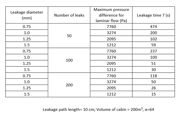
The analysis above suggests that the leakage pipe model might form a useful tool for the interpretation of the current empirical methodology. For a pipe flow, the boundary between the laminar flow range range (when the friction factor is a function of Reynolds number) and the turbulent flow range (when the friction factor is constant) is at a value of Reynolds number of around 2000. It is straightforward, using the above equations, to calculate the pressure difference that results in a Reynolds number of 2000 for different leakage geometries. Typical values are given in the table below. It can be seen that for leakage diameters between 0.75 and 1.5mm, the value of pressure difference for the transition from laminar to turbulent flow falls from 7.7 kPa to 1.2 kPa. Typical pressure transient in tunnels have maximum values of 2 to 3 kPa. There is thus a possibility that for larger leakage holes, the laminar flow pipe flow methodology (equation 12) might not be applicable and an equation of the form of equation 10 might need to be used. In this case, the concept of leakage time is similarly not valid. The table also shows leakage times for each of the cases considered, and these can be seen to fall between 15 and 500 seconds. These all fall within the range measured in experiments, and suggests equation (12) might be a useful method for relating geometric leakage characteristics to leakage time