Preamble

Since the publication of the book Train Aerodynamics – Fundamentals and Applications in 2019, I have published brief annual reviews of published papers in the field of train aerodynamics. Last year, in response to a plethora of poor quality papers, and the increasing use of sophisticated CFD techniques to tackle somewhat trivial problems, I changed the format slightly and presented brief comments on the ten “best” papers published in 2021. This seems to have been a popular format and has attracted almost 400 views in the last year, so I will repeat it this year. The concept of “best” is of course a wholly subjective one, and in reality, I have chosen the papers that follow for a number of reasons – their intrinsic quality, the fact that they address novel issues, or that the subject matter simply interests me. There are no doubt others I could have included. Nine out of the ten come from the Journal of Wind Engineering and Industrial Aerodynamics, which seems to have established its place as the leading journal in this field.

2022 seems to have been the “year of the wind fence” with a number of papers looking at the effectiveness of wind fences of different types and in different locations in protecting trains from cross winds, using both computational and experimental techniques. Although most of these have been competently carried out within their limitations, to choose just one for the following list would have been difficult, and I have thus chosen not to include any.  The papers that are presented are arranged in a number of sections that correspond to Chapters in Train Aerodynamics – Fundamentals and Applications – pressure transients (2 papers), pantographs (1), trains in high winds (3), trains in tunnels (3) and emerging issues (1).

Finally, on a personal note, it has now been five years since I retired from the University of Birmingham, and I am very conscious that I am to some degree losing contact with the latest developments in the rail industry. Thus, whilst I will continue to keep an eye on train aerodynamics papers and may well comments on them individually in this blog, this will be my last annual review of the field. Unless of course I change my mind.

Pressure transients

600 km/h moving model rig for high-speed train aerodynamics

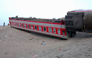
A maglev train with a speed of 600 km/h or higher can fill the speed gap between civil aircrafts and wheel rail trains to alleviate the contradiction between the existing transportation demand and actual transport capacity. However, the aerodynamic problems arising due to trains running at a higher speed threaten their safety and fuel efficiency. Therefore, we developed a newly moving model rig with a maximum speed of 680 km/h to evaluate aerodynamic performance of trains, thus determining the range of the aerodynamic design parameters. In the present work, a launch system with a mechanical efficiency of 68.1% was developed, and a structure of brake shoes with front and rear overlapping was designed to increase the friction. Additionally, a device to suppress the pressure disturbances generated by the compressed air, as well as a double track with the function of continuously adjusting the line spacing, were adopted. In repetitive experiments, the time histories of pressure curves for the same measuring point are in good agreement. Meanwhile, the moving model test and full-scale experimental result of maglev trains passing each other in open air are compared, with an error less than 4.6%, proving the repeatability and rationality of the proposed moving model.

This paper is mainly concerned with a description of a new 600 km/h moving model rig at Changsha in China. It is a remarkable piece of equipment, with sophisticated firing and braking systems. The development costs must have been significant. Having worked with moving model rigs in the past, I know that they can be prone to continual minor breakdown and breakages, particularly at high speeds, and it would be nice to know how reliable the new rig is, how many runs can be achieved in a day and so on. From the picture showing the maglev model that was used, there can already be seen to be signs of damage! The experimental results that are shown are not particularly novel, and one wonders if the equivalent results could not have been obtained on lower speed rigs and then scaled by (velocity)². But nonetheless the authors (all seven of them) are to be congratulated on their efforts

Characteristics of transient pressure in lining cracks induced by high-speed trains.

Rapidly changing pressure waves in the tunnel can aggravate the crack propagation and cause concrete blocks to fall off, posing a threat to trains. Therefore, the influences of aerodynamic pressure on the lining cracks should be considered for high-speed railway tunnels in service. In this paper, the governing equations of air in cracks were derived based on the conservation of mass, momentum, and energy, which was verified by numerical simulations using the software FLUENT. The proposed model was used to analyze the influence of train speed and crack shape on the pressure distribution, peak value and pressure waveform in the crack. Subsequently, the crack tip damage was calculated. The results show that the abrupt change of pressure can amplify the pressure and damage of the crack tip, which can be aggravated by the increase of train speed and crack mouth width.

I found this a really interesting paper that addresses an issue that has not been considered in the past – the amplification of tunnel pressure transients within cracks in the concrete lining of tunnels leading to further damage and crack growth. It is a very neat combination of a theoretical approach informed by CFD work, that leads into a structural damage assessment. Clearly the authors have given considerable thought to the issue and have used the analytical and computational tools at their disposal wisely and intelligently.

Pantographs

Influence of train roof boundary layer on the pantograph aerodynamic uplift: A proposal for a simplified evaluation method

The mean contact force between pantograph collectors and contact wire is affected by the aerodynamic uplift generated by aerodynamic forces acting on pantograph components. For a given pantograph geometry, orientation and working height, aerodynamic forces are strongly influenced by the position of the pantograph along the train roof, since an aerodynamic boundary layer grows along the train. This paper shows the experimental results of aerodynamic uplifts of full-scale pantographs located at four different positions along the roof of a high-speed train and adopts CFD simulations to examine the effect of the boundary layer velocity profile on the measured experimental forces. It is quantitatively demonstrated that the same pantograph located at different positions along the train roof can show relevant differences in the aerodynamic uplift, only due to the different flow characteristics. Moreover, a new simplified methodology is proposed to evaluate the aerodynamic uplifts at different positions of the pantograph along the train. Results of the proposed methodology are validated against full scale experimental results and full CFD simulations exploiting the complete model of the pantograph installed on the train roof.

This paper addresses an issue that has long been ignored – how the varying nature of the boundary layer on the train roof affects the aerodynamic performance of pantographs. In the past the aerodynamic coefficients have been assumed not to vary wherever the pantograph was placed in relation to the train nose. It represents a very elegant combination of large-scale wind tunnel experiments and CFD analysis, exploiting the strength of both methodologies, and leads to a straightforward and practical design methodology.

Trains in high winds

Wind tunnel test on the aerodynamic admittance of a rail vehicle in crosswinds

The aerodynamic admittance of a rail vehicle was investigated by wind tunnel test. Aerodynamic force was measured in the cases of three typical railway structures, including on the flat ground, above an embankment, and on a bridge, under two turbulent flow fields. First of all, three-component aerodynamic coefficients of the vehicle on each structure were obtained under uniform flow with respect to three wind attack angles and four wind direction angles. Secondly, the aerodynamic forces on the vehicle and the corresponding wind speed were evaluated to establish an aerodynamic admittance function of the vehicle. The aerodynamic admittance of the rail vehicle approximated a constant value in the low-frequency domain, but decreased with the reduced frequency increasing. The effects of the different reduced frequencies on the drag are greater than the lift admittance of the vehicle, while moment admittance stays steady-state. Finally, in order to reflect the unsteady characteristics of the buffeting force on the vehicle, the aerodynamic admittance functions of the vehicle were fitted to the expression of the frequency response function of a mass-spring-damping system, which was then verified. Furthermore, the effects of flat terrain and mountainous terrain were investigated, revealing that the influence of turbulence intensity on aerodynamic admittance is significant.

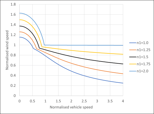
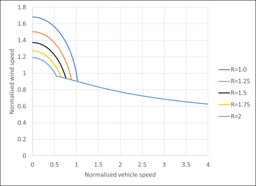
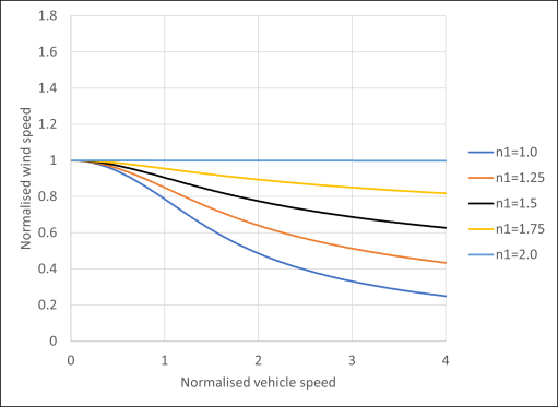
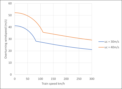
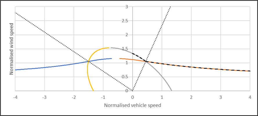
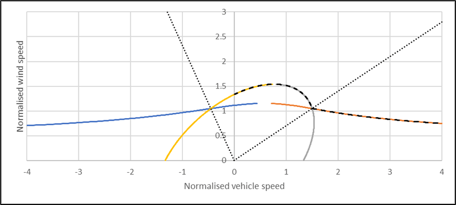
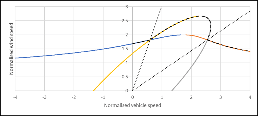
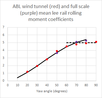
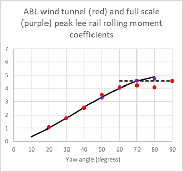
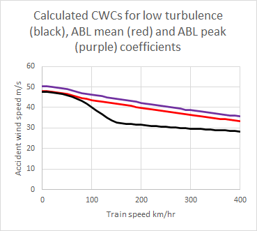
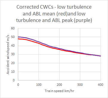
This experimental paper is the companion of a more theoretical one that was also published in 2022. This theoretical approach to describing aerodynamic admittances is based on work that I carried out in 2010, and it is good to see it much more fully investigated experimentally than myself and my co-workers were able to achieve at the time, with high quality aerodynamic admittance data being obtained for a range of turbulence simulations, and infrastructure and train geometries. There is more work to do however, in investigating just how important the concept of aerodynamic admittance actually is in train overturning calculations and how does its use affect the magnitude of the crosswind characteristics or CWCs (plots of accident wind speed against vehicle speed). The limited work myself and colleagues carried out on this a decade ago as we were developing a simple analytical framework for CWCs would suggest the effect is small, but it would be good to quantify this, and the results outlined in this paper would enable this to be done.

Impact of the train-track-bridge system characteristics in the runnability of high-speed trains against crosswinds – Part I: Running safety

This paper studies the influence of different factors related to the structure-track-vehicle coupling system in the train’s stability against crosswinds, namely the bridge lateral behaviour, the track condition and the train type. With respect to the former, a parametrization of an existing long viaduct with high piers has been carried out to simulate different lateral flexibilities. The study concluded that the bridge’s lateral behaviour has a negligible impact in wind-induced derailments. Dynamic analyses considering four scenarios of track condition, ranging from ideal to poorer condition, but still within the limits stipulated by the codes, have also been carried out, leading to the conclusion that the track irregularities influence the running safety mainly on the higher train speed levels. This is due to the fact that the Nadal and Prud’homme indexes strongly depend on the wheel-rail lateral impacts, which become more pronounced for higher speeds and under poorer track conditions. Finally, four different trains have been adopted in the study to cover a wide range of vehicles. The results proved the importance of carefully considering the trains used in the analysis, since the train’s weight may vary significantly, leading to considerable different results in terms of vehicle’s stability against lateral winds.

This is the first of a two-part paper that considers the effect of various system characteristics on train behaviour in cross winds. This paper considers the safety issue, whilst its companion considers passenger comfort issues. The analysis uses simulations of wind fields, with a sophisticated MDOF train dynamic model and looks at the effect of bridge flexibility, track roughness and train type. With regard to the former, the effects on the calculated CWCs is small. Whilst this calculation is for a concrete viaduct, the results must cast considerable doubt on the analysis of a plethora of recent papers that have considered the movement of trains over bridge of different types, using highly complex methodology to describe bridge vibrations – was such complexity really required? The effect of track roughness on CWCS was shown to be somewhat more significant and is an issue that perhaps needs to be taken into account in any future work in my view. Finally, and intriguingly, the authors show that in some instances the Prud’homme derailment criterion is critical rather than the train stability criterion and suggest that this effect ought to be taken into account in the development of CWCS. This is a significant paper, and, with seven authors, shares the prize for most contributors in this selection. They are all to be applauded!

Numerical study of tornado-induced unsteady crosswind response of railway vehicle using multibody dynamic simulations.

The tornado-induced unsteady crosswind responses of railway vehicles are investigated by using multibody dynamic simulations. Firstly, a tornado-induced aerodynamic force model is proposed by using the equivalent wind force method and the quasi-steady theory and validated by the experimental data. The Uetsu line railway accident caused by tornado winds on December 25, 2005 is then investigated by the proposed tornado-induced aerodynamic force model and the multi-body dynamic simulation. The predicted accident scenes show favorably agreement with those obtained from the accident survey when the maximum tangential velocity of tornado is around 41 m/s and the core radius is 30m. Finally, the dynamic amplification factor (DAF) for railway vehicles in tornado winds is systematically studied and it increases as the passing time decreases. It is found that the DAF can be effectively suppressed as the damping parameters increase while it decreases slightly as the natural frequency increases. A simple method to predict the DAF is also proposed based on simulation results.

This paper addresses an ongoing issue in the study of the effect of cross winds on trains – is the quasi-steady methodology adequate or are more complex models required – this time in the context of vary rapidly varying tornado loading. In the analysis the use of the discontinuous Rankine model (without radial inflow) and Burgers Rott model (which was used way outside its low Reynolds number region of applicability) somewhat limits the adequacy of the analysis, but probably not in a very significant way. The modelling is calibrated using a low speed moving model experiment. The use of the dynamic model enables significant details of the overturning process to be revealed, and shows that for rapid changes in flow velocity, there are significant overshoots in train forces from the quasi-steady values. I do wonder however, in view of the fact that tornado wind field modelling is a very uncertain procedure (and likely to remain as such) whether the complexity of the use of dynamic models is actually justified. The jury is still out on this issue I think.

Trains in tunnels

Micro-pressure wave radiation from tunnel portals in deep cuttings

The reflection and radiation of steep-fronted wavefronts at a tunnel exit to a deep cutting is studied and contrasted with the more usual case of radiation from over-ground portals. A well-known difference between radiation in odd and even dimensions is shown to have a significant influence on reflected wavefronts, notably causing increased distortion that complicates analyses, but that can have practical advantages when rapid changes are undesirable. Likewise, micro-pressure waves radiating from the portal into a cutting are shown to exhibit strong dispersion that does not occur in the corresponding radiation into an open terrain. In the latter case, formulae that represent the behaviour of monopoles and dipoles are commonly used to estimate conditions beyond tunnel portals, but no such simple formula exists (or is even possible) for cylindrical radiation that is characteristic of MPWs in cuttings. An important outcome of the paper is the development of an approximate relationship that predicts the maximum amplitudes of these MPWs with an accuracy that should be acceptable in engineering design, at least for initial purposes. The formula shows that peak pressure amplitudes decay much more slowly than those from an overground portal, namely varying approximately as r 0.5 compared with r 1, where r denotes the distance from the portal.

This paper describes a thoughtful, analytical study that addresses the effects of deep cuttings at the exit of tunnels on the reflected and transmitted pressure waves. It is shown that the reflected waves take longer to develop and are more spread out than with a tunnel outlet on level ground and that the radiating pressure wave (the MPVs) decay much less rapidly. The paper gets to the heart of the basic assumptions underlying tunnel pressure wave analysis and brings to light issues that users of commercial software need to be very aware of.

Experimental study on transient pressure induced by high-speed train passing through an underground station with adjoining tunnels

Transient pressure variations on train and platform screen door (PSD) surfaces when a high-speed train passed through an underground station and adjoining tunnel were studied using a moving model test device based on the eight-car formation train model. The propagation characteristics of the pressure wave that was induced when the train passed through the station and tunnel at a high speed were discussed, and the effects of the train speed and station ventilation shaft position on the surface pressure distribution of the train and PSDs were analyzed and compared. The results showed that the pressure fluctuation law is different for the train and PSD surfaces, and the peak pressure increases significantly with an increase in the train speed. Ventilation shafts changed the pressure waveform on the surface of the train and PSDs and greatly reduced the peak pressure. A single shaft at the rear end of the platform and a double shaft at the station had the most significant effect on relieving transient pressure on the surface of the train and PSDs, respectively. Compared with the case with no shaft, these two shafts reduced the maximum amplitude pressure variation of the train and PSD surfaces by 46.3% and 67.4%, respectively.

This paper describes a nicely set up and carried out series of experiments using a moving model rig. The situation that is considered (an underground station in a high-speed tunnel network) is quite generic and could form a useful test case for airflow calculation methods. The effect of air shafts on reducing pressures is very clear. It would have been nice to see more variations of air shaft geometry in the experimental programme, but the authors probably felt they had more than enough to do.

Field test for micro-pressure wave reduction measurement by area optimization of windows of tunnel hoods.

The air compression of a high-speed train entering a tunnel results in micro-pressure waves (MPWs), which can cause environmental problems. To mitigate MPWs, tunnel hoods with discrete windows are installed at the tunnel entrances. By properly adjusting the window conditions, the efficiency of the tunnel hood in mitigating MPWs can be enhanced. Per Japanese convention, window conditions are optimized by changing the opening/closing pattern in the longitudinal direction (pattern optimization). The optimization pattern of the windows is fundamentally different if there is a change in the train speed, train nose length, the relative position between the train and the windows, or the train nose shape. Therefore, for extremely long tunnel hoods, the optimal state of the windows is almost impossible to detect numerically or experimentally using pattern optimization. In this study, we realized a rapid and simple optimization of the windows of the tunnel hood (i.e., area optimization) for mitigation of MPWs by field measurements. The result demonstrated that the area optimization considerably helps in mitigating the MPWs, despite the simplicity of the procedures.

To reduce MPW magnitudes, the initial gradient of the pressure waves caused by train entry into the tunnel need to be minimised (since these steepen along the tunnel, with steeper waves producing stronger radiated MPWs at the outlet). One way of doing this is to design a variable area entrance hood, with openings along the side so that the pressure wave builds up gradually. The optimisation of these openings has in the past been somewhat hit and miss, and it difficult to know what is the optimal configuration. This paper describes a simple optimization methodology and presents a series of quite ambitious full-scale experiments to validate this methodology.  The final result is a very simple but effective arrangement of openings which represents the best that can be achieved.

Emerging issues

Diffusion characteristics and risk assessment of respiratory pollutants in high-speed train carriages

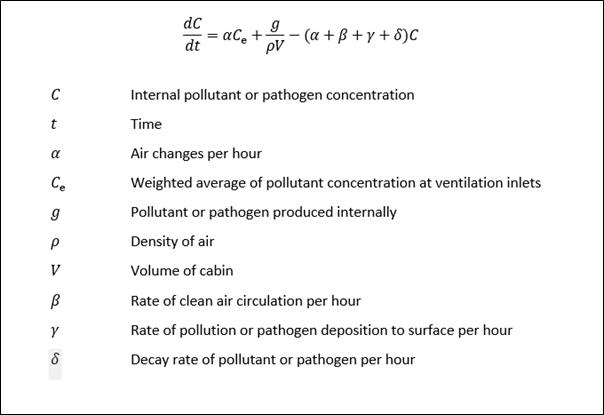
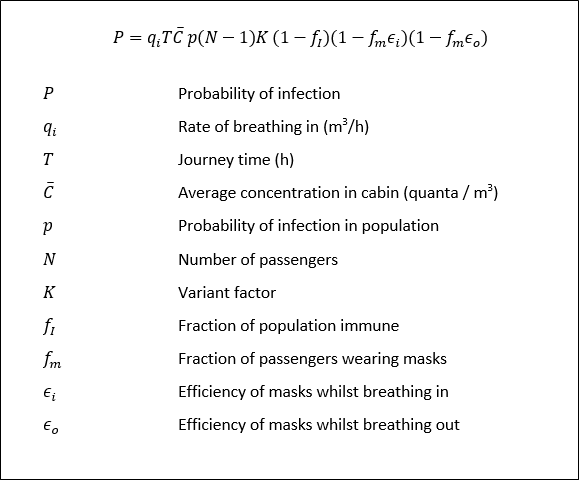
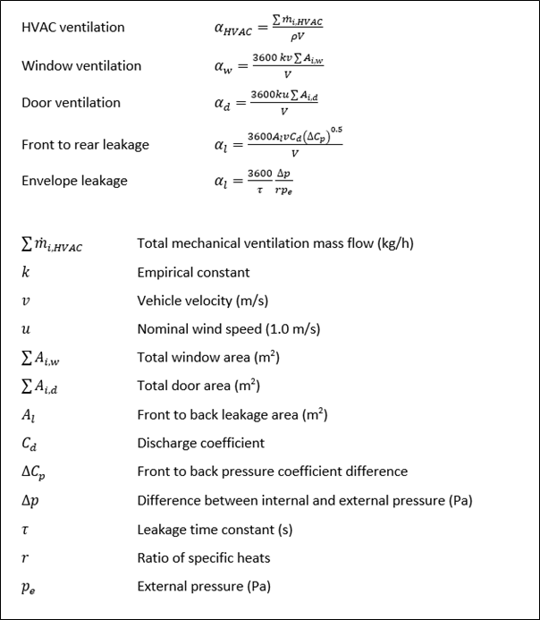
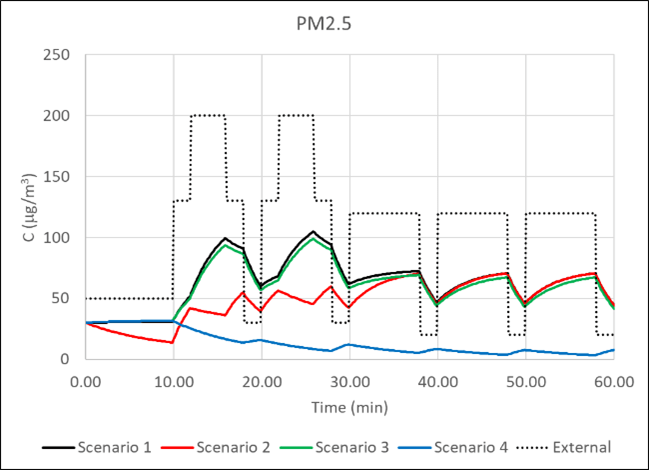
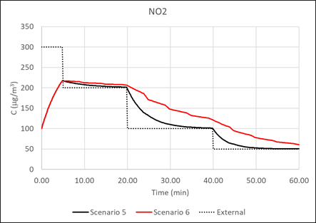
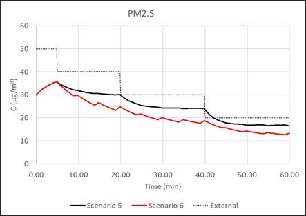
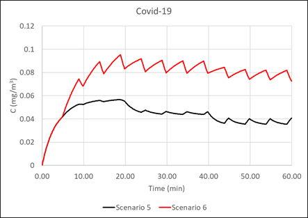
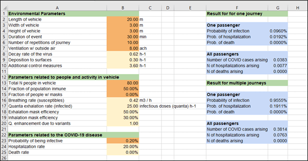
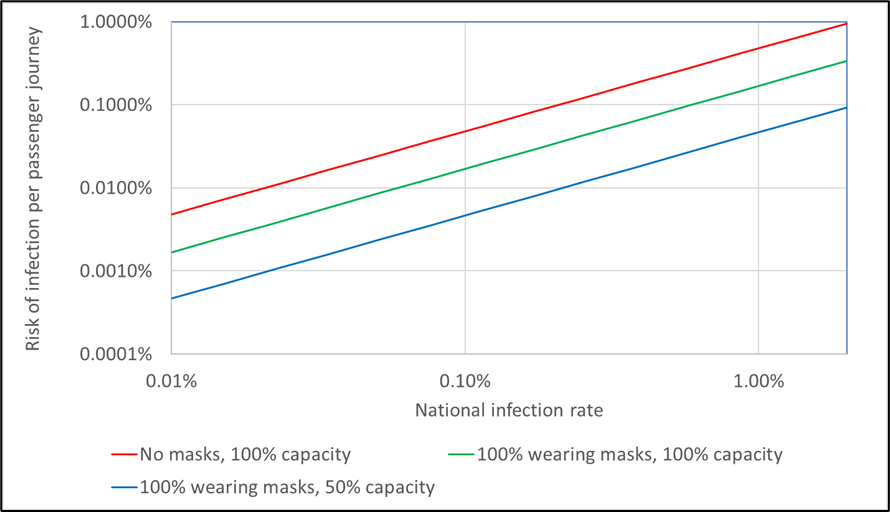
Due to the density of people in the cabins of high-speed trains, and the development of the transportation network, respiratory diseases are easily transmitted and spread to various cities. In the context of the epidemic, studying the diffusion characteristics of respiratory pollutants in the cabin and the distribution of passengers is of great significance to the protection of the health of passengers. Based on the theory of computational fluid dynamics (CFD), a high-speed train cabin model with a complete air supply duct is established. For both summer and winter conditions, the characteristics of the flow field and temperature field in the cabin, under full load capacity, and the diffusion characteristics of respiratory pollutants under half load capacity are studied. Taking COVID-19 as an example, the probability of passengers being infected was evaluated. Furthermore, research on the layout of this type of cabin was carried out. The results show that it is not favorable to exhaust air at both ends, as this is likely to cause large-area diffusion of pollutants. The air barrier formed in the aisle can assist the ventilation system, which can prevent pollutants from spreading from one side to the other. Along the length of the train, the respiratory pollutants of passengers almost always spread only forward or backward. Moreover, when the distance between passengers and the infector exceeds one row, the probability of being infected does not decrease significantly. In order to reduce the probability of cross infection, and take into account the passenger efficiency of the railway, passengers in the same row should be separated from each other, and it is best to ride on both sides of the aisle. In the same column, passengers only need to be separated by one row, and it is not recommended to use the middle of the carriage. The number of passengers in the front and back half of the cabin should also be roughly the same.

This is an interesting and important paper, arising of course out of the recent pandemic. Through the use of reasonably straightforward CFD methodology, the spread of pathogen from any point within a railway carriage to any other point can be calculated, and from this the probability of infection can be ascertained. This methodology may have widespread future use and can be used to inform passenger loading configurations with to minimise infection probabilities. The calculations were restricted to likely infection from an infected passenger in a small number of locations. There is no reason why the number of locations should not equal the number of possible passenger conditions and a matrix produced on of infection in seat i due to an infected individual in seat j, which would enable a fuller picture of infection rates to be developed.

Preamble

In January 2020 and January 2021, I posted quite lengthy blog posts that attempted to collate all the published papers in train aerodynamics over the previous year  – see here for the 2020 post and here and here for the two part 2021 post. . These were intended as supplements to the book “Train Aerodynamics – Fundamentals and Principles” published in 2019. These blog posts have been quite widely read. At the time of writing (mid-January 2022) the 2020 post has had 190 views and the two parts of the 2021 post 129 and 70 views. It had been my intention to do something similar for the papers published in 2021. However, I have changed my mind on this, and instead will take a different approach in this post. My reasons for this are twofold.

• The number of papers in the field continues to proliferate and, quite frankly, many of them are of poor quality. This seems to be driven by the need, in some jurisdictions, for research students to publish papers in order to be awarded a PhD. This inevitably encourages a low standard of output. Also, I have noticed an increasingly disturbing trend, whereby when a paper is rejected by one of the higher quality journals, it is submitted in much the same form to other journals with less impact.  I have seen a number of such papers sent to me to review by different journals – and on two occasions in 2021 I have been sent the same paper by three journals. Obviously I have little influence on how researchers submit papers, other than through the normal reviewing process, but there seems to me no reason to give such papers the benefit of a mention in any comprehensive annual compilation.
• The use of CFD techniques in train aerodynamics, which is proliferating at the same rate as the number of papers, is giving me increasing concern. CFD techniques ranging from RANS to LES are exceptionally useful tools in all fluid dynamics research and the same applies in the train aerodynamics field. But they are as much tools as any physical model tests and need to be used and interpreted very carefully. There are many investigators who do just that, including colleagues in my own institution. However, I fear that that is not always the case Specifically, the use of such techniques is in many circumstances becoming divorced from practical reality. There is a tendency to apply quite high level, but inflexible, CFD methods (such as IDDES) to look at quite trivial problems where much simpler methods could have given equivalent answers over a wider parameter range. And in the consideration of the results from these calculations, there is often little appreciation of the uncertainty that is attached both to the CFD results themselves (for example I have seen the percentage changes in predicted drag given to two decimal places) or in relation to full scale reality, where the uncertainties are multiplied by an order of magnitude or more.  Further the results of the CFD calculations are often massively over-analysed. For example, in studies of cross wind effects on trains, I have come across papers where the predicted wake systems are analysed in very great detail, with little realisation that any such systems cannot exist in reality due to the (unsimulated) large scale turbulence in the approach flow field – as of course is the case with many wind tunnel tests. The same can be said of the analysis of many other applications. Again, there is little I can do to influence these trends, but I see no reason to publicise such work any further in blog posts.

In the light of such developments, in this post I will not present a comprehensive compilation of all the train aerodynamics papers from 2021 but will rather choose a much smaller number (ten in total) which I believe are of particular significance and likely to influence the field in the future. These are spread across the range of train aerodynamic applications including train drag studies, trains in tunnels, crosswind effects and emerging issues. The choice of what to include is of course to some degree subjective and mirrors my own interests, but I hope that readers find it of interest.

Train drag studies

On the influence of Reynolds number and ground conditions on the scaling of the aerodynamic drag of trains. Tschepe et al (2021)

Very often the effect of Reynolds number on train drag measurements or calculations is broadly ignored provided that the Reynolds number is “high enough”. This is of course not adequate, as the skin friction component of drag must vary with Reynolds number throughout the parameter range – see for example my historically rather crude analysis of the problem from 1991. This paper, drawn from the doctoral work of Tschepe) presents the results of a thorough experimental and analytical investigation into this effect, using the results from water towing tank experiments. These experiments are quite novel and deserving of attention in their own right. The three-dimensional nature of the train boundary layer is clear, and the effect of ground roughness (ie sleepers and ballast) is shown to be of some importance (see also my blog post here). A simple analytical approach, based on flat plate theory, allows a correction method to be developed for extrapolating low Reynolds number results to full scale conditions.

A field study on the aerodynamics of freight trains Quazi ei al (2021)

This paper presents the results of full-scale measurements of the pressure drag of a freight container during a typical journey. As such it provides a basic benchmark for further studies. The technique is of interest in its own right, but the basic result, that, despite the container not having other containers immediately in front and behind it, the drag coefficient is much lower than that found in other full-scale, physical model and numerical calculations is of considerable interest. The authors suggest that this is because of the container position much further down the train than in other measurements, as well as other modelling issues. The results perhaps give pause for thought about the measurement of train drag from wind tunnel tests or CFD calculations.

Tunnel aerodynamics

Influence of air chambers on wavefront steepening in railway tunnels. Liu et al (2021)

The phenomenon of micro-pressure waves (sonic booms) emitted from tunnel portals has been much studied in recent years. These are caused by the steepening of the train nose pressure wave as it passes along the tunnel, resulting in a steep wave at the tunnel exit that is not wholly reflected with some energy being transmitted out of the tunnel in the audible frequency range. The standard method for the amelioration of such effects is through the use of tapering tunnel entry portals, that reduce the initial (and thus the final) steepness of the waves. Such portals can be quite long and extend some way out of the tunnel, and indeed can be quite expensive. This paper investigates an alternative to such portals – the distribution of air chambers along the length of the tunnel that in principle reduces the steepening of the pressure wave. Using a relatively straight forward gas dynamics analytical model, the authors show that suitably designed chambers can remove the dependence of the exit wave on the steepness of the inlet wave. Guidance is given for appropriate chamber volumes and the resistance of the connectors between the chambers and the tunnel. Overall, the method has much potential for future tunnel design.

Virtual homologation of high-speed trains in railway tunnels: A new iterative numerical approach for train-tunnel pressure signature. Brambilla et al (2021)

The standard methodology to investigate the passage of pressure waves along tunnels is to use full-scale measurements to measure the pressure wave system on train entry, and then to use data from those measurements to predict the pressure wave along the length of the tunnel using one dimensional gas dynamics methods. The latter can be run many thousands of times to investigate a range of operational conditions. Clearly the required full-scale tests are expensive and complex. Recently some full CFD calculations of the flow along tunnels have been published using sliding grids, which are again highly complex and computer resource requirements limits their use to just one or two conditions. This paper presents a combined methodology where CFD calculations using a standard fixed grid are carried out to measure the pressure characteristics at train inlet to the tunnel, and these are then used in one dimensional methods. The methodology has been validated against an extensive full scale data set. Its relative cheapness and flexibility means that it has the potential to become widely used within the industry.

Semi-empirical model of internal pressure for a high-speed train under the excitation of tunnel pressure waves. Chen et al (2021)

This paper looks in detail at the development of internal pressures within train cabins in tunnels. Using a combination of commercial CFD and finite element analysis, together with simple models of internal ventilation flow, the authors looked at pressure changes due to body deformation, pressure transmission through gaps in the train envelope and transmission through the air ducts of HVAC systems. Body deformation has little effect (unsurprisingly in my view) with the balance between gap and duct transmission varying depending on the degree of opening of the latter. Whilst the analysis is complex, the results should be of interest in describing a methodology that could ultimately be applied quite straightforwardly in design.

Pressure fluctuation and a micro-pressure wave in a high-speed railway tunnel with large branch shaft. Okubo et al (2021)

This paper describes an extensive experimental programme using a moving model facility that looked at the micro-pressure waves that occur as a result of the junction between the main tunnel and large branch tunnels with similar diameter (which would be used for passenger evacuation). The results are skillfully interpreted through the use of analytical models and show that in some instances the micro pressure wave emitted from the branch tunnel can be of greater magnitude than that omitted from the main tunnel. Both the physical and analytical modelling methodology have potential use for the design of complex branching tunnel systems.

Trains in crosswinds

Influence of the railway vehicle properties in the running safety against crosswinds. Heleno et al (2021)

I include this paper with some temerity, as I am named as an author – albeit the last one. However, my role was very minor, and mainly involved discussions on some technical details and proof reading the final draft (although they all contribute to my long term aim of getting to 200 journal publications before my demise!). This paper considers the effect of various railway vehicle properties on the overturning risk of a rail vehicle. It uses realistic vehicle dynamic and track roughness models and generates realistic time series of wind speed from wind statistical parameters. It is more rigorous in its modelling than the current method used in the CEN code, which uses a very simplified wind gust model. A thorough parametric analysis of the various vehicle parameters is carried out. In my view the major point to emerge is the lack of sensitivity of the calculated overturning wind speeds and safety risk to variations in the train suspension parameters. In principle this could lead to much simpler models for the CEN safety assessment than are used at present, where full dynamic modelling is required. This is personally satisfying as I have been arguing this very point for the last 10 to 15 years – see the discussion in this post from 2020.

Emerging issues

CWE study of wind flow around railways: Effects of embankment and track system on sand sedimentation. Horvat et al (2021)

I include this paper because it contributes to what I believe to be an important emerging issue as railways are developed in arid conditions – sand sedimentation over railway tracks. It is a straightforward CFD study of flow patterns over different railway track geometries that calculates wall shear stresses and used these to define potential regions of erosion and sedimentation. It lays the foundation for future work – possibly to integrate sediment modelling into the CFD calculations.

Investigation on flow field structure and aerodynamic load in vacuum tube transportation system. Zhong et al (2021)

This paper is a detailed CFD analysis of the flow around vacuum tube vehicles using IDDES techniques. Because of the enclosed nature of the vehicles and the well-defined geometry, this is a case where one would expect good accuracy from such calculations. Also of course the issues cannot be easily addressed by physical modelling techniques. Both subsonic and supersonic flows are considered, the nature of the flow field elucidated, and vehicle drag calculated. The results form a useful addition to the publicly available body of knowledge about the flows around such vehicles that can be used in further development of the concept. That being said, it is my firm view that, fascinating as the aerodynamics of the system might be, vacuum tube systems will not meet with wide adoption due to simple operational constraints – primarily the low capacity in comparison to conventional high speed rail systems.

General

Railway applications – Aerodynamics – Part 7: Fundamentals for test procedures for train-induced ballast projection. CEN (2021)

This is not a paper, but rather the latest offering from the CEN working group on Aerodynamics that looks at the issue of ballast flight beneath high-speed trains. It contains a wealth of information of the issues involved, economic aspects of the damage caused by ballast flight, current national practices and possible ways forward in terms of homologation. It is well put together and forms a very useful basis for further work in the field.

When considering the effect of crosswinds on a new train, an obvious first step is to obtain data on the aerodynamic force and moment coefficients, usually through the use of wind tunnel tests, with the forces and moment coefficients being measured for a range of yaw (wind) angles from 0 to 90 degrees. This process however is not quite as straightforward as it sounds. The conventional approach is to use static models in a low turbulence wind tunnel. This approach of course models neither the relative motion between the train and the ground, nor the effects of atmospheric turbulence. It does however have the merits of simplicity and convenience. The conventional argument often used to justify this approach is that for high-speed trains, the relative motion between the train and the wind leads to the train experiencing low levels of turbulence. Whilst this is the case to some extent, it is not a wholly adequate argument. Figure 1, from Train Aerodynamics – Fundamentals and Applications (TAFA), shows how the turbulence length scale, turbulence intensity and velocity shear relative to the train vary with train speed for a 90 degree cross wind. Values are given as ratios of the values when the train is stationary. It can be seen that even at 400 km/h, the train still experiences a turbulence intensity of around 30% of its stationary value, which one might expect to have a not insignificant effect on the flow around the train,.

Figure 1 Variation of relative values of turbulence intensity (black), turbulence length scale (red) and shear (green) with train speed for a 90 degree cross wind (from TAFA)

An alternative approach would be to use a wind tunnel simulation of the atmospheric boundary layer in which to measure the train forces and moments. This of course is only really applicable to stationary trains. On the basis of figure 1, I argued in TAFA that low turbulence wind tunnel tests would be best for train speeds greater than 200 km/h and atmospheric boundary layer tests would be best for train speeds below that value – but that of course represents rather a messy compromise. And both methods fail to address the issue of train / ground relative motion.

So what are the alternatives? The first might be thought to be the use of CFD to properly model both atmospheric effects and train / ground motion. However, the simulation of a realistic scenario requires complex CFD methodologies (usually DDES) with very complex domain boundaries that include the specification of atmospheric turbulence. The calculation of the flow field for just one yaw angle takes several weeks on supercomputer systems, and in reality CFD calculations of this type tend to mirror the low turbulence wind tunnel tests.

In physical model terms, two alternatives present themselves. The first is the measurement of cross wind forces and moments on a moving model rig such as the TRAIN Rig owned by the University of Birmingham.  Again, the experimental issues are formidable. The use of force balances within moving model rigs is not straightforward, and measurements of this type are usually made through the measurement of surface pressures with internal transducers, which because of transducer size and the need to carry out multiple runs to obtains stable average pressures requires multiple runs, with different pressure positions at any one yaw angle – a very tedious and complex process. An alternative would be to carry out conventional wind tunnel tests, but with a range of different turbulence simulations, each simulation being valid for one train speed only. The thought of such tests is enough to make wind tunnel operators consign it to the rubbish bin without much hesitation.

But the issue is important. Figure 2 shows three different sets of lee rail rolling moment coefficients for the Mark 3 coach, the GB benchmark vehicle that has run on exposed lines for many decades without incident. The three sets of coefficients are obtained from low turbulence wind tunnel tests; tests with an atmospheric boundary layer simulation with the coefficients formed from the mean values of measured forces and velocities; and those obtained from similar tests but with the coefficients formed from one-second peak values of forces and velocities (from Measurements of the cross wind forces on trains). The atmospheric boundary layer results are shown together with corresponding full scale results from field measurements on a real train. There can be seen to be significant differences between the three curves, particularly in the low yaw angle range which is important at high train speeds, with the low turbulence values being significantly above the atmospheric boundary layer values and the peak values being below the mean ones. If these coefficients are used to obtain cross wind characteristics (CWCs), which are plots of accident windspeed against vehicle speed, as outlined in another post and in TAFA chapter 11 and in a recent blog post, then the differences in acceptable windspeeds can be seen to be significant, particularly in the speed range around 200 km/h – see figure 3. Note that this plot shows train speeds of up to 400 km/h, which is wholly unrealistic for the Mark 3 coach – and certainly I wouldn’t care to be in one travelling at that speed! – but serves to illustrate the lack of agreement between the CWCs calculated using different moment coefficients. The difference in CWCs can be expected to make a significant difference to the calculation of accident risk, or to any operational restrictions that might be imposed, with the low turbulence results giving higher risk values and more severe restrictions.

Figure 2. Lee rail rolling moment coefficients for Mark 3 coach

Figure 3 Crosswind characteristics for Mark 3 coach

I have to admit this is a problem that I have been mulling over on and off for many years (which gives a rather sad picture of the life I lead I fear). My thoughts have been basically around the idea of how to obtain representative force coefficients to allow for the major effect of atmospheric turbulence at low train speeds and the much smaller effect at high speeds, perhaps by some interpolation of the low and high turbulence coefficients. This is not simple however, as there is no direct correspondence between variation of these coefficients with yaw angle and variation with train speed.

But there is perhaps another way – and that is to consider not the force and moment coefficients, but rather the CWCs shown in figure 3. It seems reasonable to me to assume that the most representative CWC would lie somewhere between the low and high turbulence characteristics, lying close to the ABL curve at low train speeds, and close to the low turbulence curves at high train speed. Thus figure 4 shows the CWCs formed from giving a variable weighting to the low and high turbulence curves at different train speeds, with a 100% weighting given to the low turbulence curves at a train speed of 0 km/h, and a 0% weighting at a train speed of 400 km/h, with a linear variation in between. More sophisticated weighting variations could be considered, but this approach is adequate for illustrative purposes. The two curves of figure 4 are for the interpolation of the CWCs calculated from the mean and peak coefficients with those obtained from the low turbulence coefficients. It can be seen that this approach significantly raises the CWCs in the mid speed range from the low speed values and will thus result in substantial risk reduction.

Figure 4. Interpolated cross wind characteristics

Up to now, I have referred to potential risk reductions in rather broad terms. It is however possible to put some numbers to these statements. Table 1 shows the accident wind speed at a train speed of 200 km/h for each of the above CWCs and the associated risk at the reference site as defined in my earlier post. For the original CWCs derived from the ABL coefficients, , the risks is of the order of 10^-7 to 10^-8, but for the CWC derived from the low turbulence conditions, the risk approaches 10^-5 – almost two orders of magnitude greater. Whilst the absolute values of risk are quite arbitrary, it is clear that the use of the low turbulence characteristic would lead to a much more pessimistic (and perhaps unrealistic) risk assessment, and lower than necessary wind speed restrictions. The interpolated CWCs give values of risk of ca little less than 10^-6, roughly midway between the atmospheric boundary layer and low turbulence values.

Table 1. Accident windspeeds and risk values for Mark 3 coach at a train speed of 200 km/h

So to conclude, the method outlined above gives a potentially realistic way of solving the problem of what type of wind tunnel test to use for train cross wind risk assessment. It requires two sets of wind tunnel experiments, one with low turbulence and one with an atmospheric boundary layer simulation, which is a more complex methodology than at present, but does not require extremely complex wind tunnel or CFD trials. The method results in lower values of calculated risk than would be the case using conventionally derived CWCs, and higher values of accident wind speeds.

Preamble

Most modern trains are “sealed” in that they are designed to minimise the leakage of air between the inside and the outside of the cabin. There are a number of reasons for this. Firstly HVAC systems require as little leakage as possible to be able to operate efficiently. Secondly, when a train passes through a tunnel at speed, it generates large pressure transients that can cause passenger aural discomfort and pain – sealing the train attenuates or even eliminates such transients in the train interior. However the sealing of trains is never perfect and some way of quantifying leakage is required, and then of calculating the internal pressure of trains for the types of external pressure field experienced as trains pass through tunnels, allowing for this leakage. This brief post looks at the standard methodology for doing this, which is essentially empirical, and compares it firstly with methods for the calculation of leakage in buildings used by ventilation engineers, which are based on the concept of an equivalent orifice, and secondly with a new method which models leakage paths as simple pipe flows. It is shown that the empirical model currently used is consistent with the new leakage pipe model, and the use of the latter enables some of the limitations of the current method to be more fully appreciated.

The railway methodology

The standard method for assessing how well a train is sealed is to pump air into the train to raise the internal pressure to a specified level and then simply to observe the decay of pressure when the pump is turned off. It is then assumed that this pressure decay follows the simple rate equation shown in equation (1), which can be solved to give the exponential decay expression of equation (2) The parameter T is a leakage time constant and can usefully be used to quantify the degree of sealing (Note that this is usually denoted by the Greek letter tau, but this website is unable to cope with Greek letters in the text). Tests are usually carried out for static trains but can in principle be carried out for moving trains, where one might expect the degree of sealing to be somewhat less than the static case due to the relative movement of different parts of the train envelope. Thus two values of the leakage time are often defined – T_static and T_dynamic.  The sealing criteria themselves vary somewhat around the world and are usually expressed in terms of a minimum time for the pressure to fall from one specified value to another. These criteria are usefully summarised in Niu et al (2020). The range of criteria effectively imply values of T of the order of 10 to 60 seconds. Once a value of T has been determined, equation (1) can be used in reverse to find how  the internal pressure varies for rapidly varying external pressures, such as when trains pass through tunnels. This usually requires a numerical solution to equation (1).

The calculation of leakage in buildings

Now the approach taken in the study of building ventilation is somewhat different. A number of authors, for example Harris (1990) developed an equation for the flow in and out of buildings with both major openings such as windows, and with a distributed minor leakage openings. For the case of leakage only, which is most analogous to the train case, the basic expression used in given in equation (3). This is effectively an equation for flow through an orifice, and the basic assumption is that the leakage area can be represented by an equivalent orifice. It is then assumed that the change in internal pressure is an adiabatic process, and thus equation (4) applies. I am not altogether sure why the process should be adiabatic rather than isothermal, but that is probably due to my lack of understanding of thermodynamics. Putting these equations together gives equation (5), which is equivalent to equation (1) except that the change in internal pressure is proportional to the root of the difference between the external and internal pressures, rather than being directly proportional.

Now the analysis that leads to equation (5) assumes that the orifice coefficient remains constant. However, at low orifice Reynolds numbers, the coefficient is known to fall significantly – see Johansen (1930) and the figure below. (I find I have rather a perverse pleasure at quoting a technical paper that is almost 100 years old!). This implies that equation (5) can only be valid when the pressure differences, and associated leakage flow rates, are quite high. To investigate this further, on the basis of the experimental results shown in the figure below, we take the discharge coefficient to vary with the square root of the Reynolds number as in equation (6). Here the Reynolds number is based on the leakage velocity v and the average diameter of a single leakage path d (which can be expected to have a very much smaller area than the overall leakage area A). After some manipulation this results in equation (7). This is of exactly the same form as equation (1), and the leakage time constant can be explicitly expressed as in equation (8).

There is still however an issue in applying this equivalent orifice analysis to the case of train leakage. From equation (3) above, the velocity through the orifice is directly related to the pressure difference, with the energy loss being described by the discharge coefficient. For the values of pressure difference across building facades, which are of the order of tens of Pascals, typical values of the discharge coefficient of around 0.6, result in velocities through the orifice are of the order of 1m/s. The pressure differences between the inside and outside of trains in tunnels however can be up to 2 or 3Pa, and an orifice type analysis would give velocities of 40 or 50m/s, which is clearly unrealistic. The discharge coefficient method therefore does not give an adequate energy loss to the leakage flow for high pressure differentials. So this type of analysis may be applicable in building ventilation, but does not seem appropriate for the consideration of train leakage. Some other framework needs to be developed to give the railway methodology for calculating leakage something other than an empirical basis.

Leakage tube methodology

As an alternative, it is possible to conceive of the leakage paths on a train as a set of equivalent pipes. Equation (3) can then be written in the form of equation (9) – which is effectively Darcy’s law for flow through a pipe. The energy loss in the system is determined by the Darcy friction factor. After some manipulation one arrives at the expression of equation (10), which is equivalent to equation (5). Now for high Reynolds numbers (> around 2000) the Darcy friction factor will be constant, and the rate of change of pressure will be proportional to the root of the pressure difference between inside and outside the train – as in the orifice flow analysis. However at low Reynolds numbers the Darcy friction factor varies inversely with Reynolds number as shown. This results in equation (11), which gives the rate of change of internal pressure as being proportional to the difference between the external and internal pressures rather than the root of the difference i.e. a similar form to the empirical equation (1). An equivalent value of the leakage time constant can be derived – equation (12). The energy loss in the system is very much greater than for an orifice flow.

Implications

The analysis above suggests that the leakage pipe model might form a useful tool for the interpretation of the current empirical methodology. For a pipe flow, the boundary between the laminar flow range range (when the friction factor is a function of Reynolds number) and the turbulent flow range (when the friction factor is constant) is at a value of Reynolds number of around 2000. It is straightforward, using the above equations, to calculate the pressure difference that results in a Reynolds number of 2000 for different leakage geometries. Typical values are given in the table below. It can be seen that for leakage diameters between 0.75 and 1.5mm, the value of pressure difference for the transition from laminar to turbulent flow falls from 7.7 kPa to 1.2 kPa. Typical pressure transient in tunnels have maximum values of 2 to 3 kPa. There is thus a possibility that for larger leakage holes, the laminar flow pipe flow methodology (equation 12) might not be applicable and an equation of the form of equation 10 might need to be used. In this case, the concept of leakage time is similarly not valid. The table also shows leakage times for each of the cases considered, and these can be seen to fall between 15 and 500 seconds. These all fall within the range measured in experiments, and suggests equation (12) might be a useful method for relating geometric leakage characteristics to leakage time

Part 1 of this review can be found here

Trains in tunnels

The most important flow parameter to be considered in a study of tunnel aerodynamics is of course the rapid change in pressure as trains pass through. A number of investigations in this area have reported in 2020. Perhaps the most significant is the full-scale investigation of Somaschini et al (2020). They measured both on track and on train pressure measurements on a high-speed Italian line. They showed the pressure transients caused by trains in tunnels were very sensitive to the initial flow conditions in the tunnel, and specifically the residual velocities caused by the passage of earlier trains. The on-train measurements consisted of the measurements of pressures around the train envelope, together with the internal pressures for both sealed and unsealed trains. The effects of train passings were also measured, and the effect of HVAC shuttering systems on internal pressures identified. This is a very substantial piece of work and provides much data that could be used for the verification of physical and numerical modelling methodologies in the future. Lu et al (2020) investigated pressure transients for trains crossing in a tunnel using RNG k-epsiilon CFD techniques and moving model experiments.  They used three of four coach trains in tunnels of varying length. The main thrust of the investigation was aimed at investigating the effect of changes in tunnel cross section. There was a respectable level of agreement between CFD and physical model tests, and the authors concluded that the optimal geometry for a reduction in tunnel section depends upon the point at which trains pass, which is of course very difficult to control in practice. Izadi et al (2020) used a simple moving model of circular train in tunnel and compared the results with standard RANS methods. Unsurprisingly there was good agreement. Although this work is in effect a repeat of work that was carried out in the 1970s and 1980s, it does have a novel aspect in that the effect of trains accelerating and decelerating was investigated.

The other major flow parameter of importance is of course the flow velocity, in the slipstream and wake of the trains. These have been investigated by two studies. Li et al (2020a) investigated the slipstreams caused by single and passing trains using URANS CFD calculations around eight coach trains passing through a tunnel roughly three times that length. Unsurprisingly they found that the slipstreams and wakes were highly complex varying both spatially and temporally. The highest velocities were in the train / wall gap or in the gap between passing trains as would be expected. Interestingly they found that the size of the longitudinal vortices in train wakes decreased as the train entered the tunnel and were constrained by the tunnel walls, although their vertical extent increased. Meng et al (2020) used IDDES CFD techniques to investigate the slipstreams and wakes in tunnel for trains with different nose shapes. A three-coach train geometry was used, with noses of variable length. It was found that the long nose shape reduced the slipstream velocities throughout the tunnel.

The reduction in strength of micro-pressure waves from tunnel outlets continues to be a topic of investigation. Luo et al (2020b) investigated this effect for mountainous terrain where there was no space for lengthy for entrance structures, looking instead at the use of cross passages near the tunnel inlet. Both moving model tests and CFD techniques were used, and good agreement was found. It was concluded, again perhaps unsurprisingly, that as many large cross passages near the tunnel entrance as possible had most effect on the strength of the MPW emitted from the tunnel. Saito and Fukuda (2020) investigated entrance stepped hoods of variable area with porous opening using acoustic theory and found that the optimal design could results in significantly shorter hoods than conventional designs.

The study of the aerodynamics of subway systems continues to develop with a number of investigations carried out. In particular there have been two full scale investigations reported. The first, by Hu et al (2020) measured airflow characteristics in the tunnels around a subway station and used the results to calibrate a network model. This model was then used to investigate the effect of different arrival and departure strategies on the air flow within stations.  The cooling load of train air flow was also investigated, in relationship to mechanical ventilation methodologies.   There were significant variations in ventilation characteristics as train operation varied, but the authors found it was possible to arrive at an optimized HVAC operation. Khaleghi and Talaee (2020) carried out full scale velocity measurements in a subway station with longitudinal ventilation of tunnels, with a novel air curtain system to control the ventilation flows within the station. The results were used to calibrate a CFD methodology, which was then used to investigate a range of ventilation and air curtain strategies studied.

Liu et al (2020b) used a standard k-omega SST CFD methodology to investigate a four-coach train accelerating to 120km/h as it left a station and entered a tunnel, and in particular made estimates of the time varying pressure and friction drag. As would be expected, the latter increased substantially on tunnel entry. Huang et al (2020) also used a standard RNG k-epsilon CFD methodology to investigate the loads on the surfaces of tunnels caused by the passage of a six-car subway train. The methodology was verified using equivalent moving model tests. The investigation showed that the loads were particularly sensitive to overall tunnel blockage and tunnel shape.

Finally, it is necessary to point out that the effect of air movement on the spread of fires in tunnels is not considered here. The interested reader is referred to Liu et al (2020c) and Peng et al (2020) for recent investigations.

Trains in crosswinds

Crosswind forces

One of the basic requirements for the study of trains in crosswinds is a knowledge of the crosswind induced forces. As pointed out in TAFA, the determination of these forces is not straightforward either experimentally or numerically. A number of authors have addressed some of these issues. Liu et al (2020d) investigated the optimum number of pressure taps on a train to obtain accurate forces and moments through pressure integration using DES methodology for a three car HST at yaw angles between six to thirty degrees, and compared their results with directly measured forces from wind tunnel tests. They found that an arrangement of 15 x 4 taps on each face of the train produced adequate results although the difference between the computed and measured force coefficient values was considerable (up to 10% for side force coefficient, and up to 20% for lift force coefficient. Interestingly they found that only between 2 and 4% of the forces were due to friction rather than pressure effects.  Huo et al (2020) investigated whether the trailing edge shape of dummy vehicle in crosswind tests (which is conventionally mounted behind the live vehicle) affected the measured forces and moments. A range of shapes were considered, from blunt ended to streamlined, using DDES-SST techniques. Little effect was found for yaw angles up to 45 degrees, but both side and lift force coefficients fell below the values for long trains at a yaw angle of 60 degrees, with the trailing edge shape making little difference. Li et al (2020b)  looked in detail at the choice of the RANS methodology embedded within the DES approach, an important issue that has not been much investigated in the past. In particular they investigated the adequacy of the one equation SA-DES approach and the two equation SST-DES approach as applied to a Class 390 train at a yaw angle of thirty degrees, for which wind tunnel data was available.  Both methods gave similar values and trends, of surface pressure but there were considerable differences in the predicted separation positions. Side force and rolling moment coefficients were similar, but lift force coefficient were very different. The authors concluded that SST-DES was the most appropriate to use.

CFD techniques were also used to investigate the effect of specific geometrical features on measured and calculated crosswind forces. Guo et al (2020b) used DDES to investigate the effect of bogie complexity on crosswind measurements and found that the rolling moment coefficients increased as bogie simulations became more complex, with a variation of around 20%.  Jiang et al (2020) carried out a DES investigation of the effect rail type in cross wind simulation. No rail, simple rail, complex rail simulations were  used. It was found that there was little effect on side force coefficients and rolling moment coefficients were only affected in the higher yaw angle range but lift force coefficients were significantly affected for all yaw angles. The results for the simplified and complex rail simulations were very similar. Maleki et al (2020) in their LES study of double stack freight in crosswind particularly investigated the effect of the gap between containers. They showed that variations in gap width had a significant effect on flow topology, which was highlighted through significant differences in mode shape appearing in a POD analysis. The flow structures that were observed included vortices from the leading windward corner of the container and longitudinal vortices from the top and bottom leeward corners. The authors were mainly concerned with the effect of crosswinds on drag, and their work illustrated the drag benefit of keeping the gaps between the containers small, which became more substantial as yaw angles increased.

Zhang et al (2020b) carried out a CFD analysis of the Chiu and Squire idealised train model at 90 degrees yaw and used various optimization schemes to optimize cross wind forces by geometric changes. They found that the changes had little effect on side forces, but that lift could be reduced by 20% by small sectional modifications. The work has little practical significance.

The investigations described above have, if only implicitly, been concerned with the crosswind forces on train due to normal, cyclonic winds. By contrast Xu et al (2020a), using DES simulations, investigated the forces on  a three-car train passing through a tornado simulation. The tornado was small in relation to the train, and there were significant scaling issues as in all such simulations. Forces were calculated for different vortex positions relative to the train, and whilst of high intensity were found to be transient and very localized. The overall representativeness of the simulated flow field in relation to real tornadoes must be questioned.

A number of investigations, usually CFD studies, have looked at crosswind forces on trains in the presence of different infrastructure geometries. Guo et al (2020c) used DDES techniques to study flow over embankments with and without trains. A three-car HST model was used, with embankments up to 7m high, with a simulation of an upstream power law profile. Both velocities and train forces and moments were measured for a range of different cases. The results are potentially very useful and need to be integrated with existing compilations of similar measurements. Wang et al (2020e) carried out a RANS study on a three-car HST to investigate the effects of ground clearance, typical embankments and viaducts and a truss bridge, at yaw angles of 30, 45 and 60 degrees. Results are presented for side and lift force coefficients for the different cases. Li and He (2020) carried out wind tunnel measurements of a train on a bridge with a ninety-degree wind and measured aerodynamic forces and moments for different angles of attack. As this angle varied across the range that might be expected in reality, significant variations in the forces and moments were observed. These results are valuable, although the authors recognize that strictly they are valid only for the bridge geometry that they studied. Zou et al (2020) used RANS SST to study the aerodynamic forces and moments on a three-car HST as it travelled into and out of an area on a bridge sheltered by a wind barrier. Very high unsteady forces were observed on both train and barrier at entry and exit. Yao et al (2020) carried out a similar RANS SST study of a train on a truss bridge and also found similar highly transient and unsteady forces. They also investigated the effect of angle of attack. Gu et al (2020) report a study of flow and forces behind corrugated wind barriers, with a wavy section of different types. Very large-scale high blockage wind tunnel tests were carried out on a train section at 90 degrees yaw, together with equivalent DES calculations. The forces on the train section varied significantly with barrier “bendiness”.

Two investigations have looked in detail at the crosswind forces on trains as they emerge from a tunnel onto a viaduct in complex terrain.  Deng et al (2020b) carried out a RANS study and found very rapid transients for all forces and moments with some significant overshoots of the equilibrium value. Wang et al (2020f) using SST k-epsilon methods looked at the effect of wind barriers at the tunnel bridge junction, comparing the transient forces with and without barriers.

Vehicle system modelling

Having determined the force and moment coefficients, the next step in addressing crosswind safety is an analysis of the vehicle / wind dynamic system. This requires some formulation to describe wind gusts. There are three basic approaches – the specification of gust magnitudes alone, the specification of a discrete gust shape, and the full stochastic representation of the wind. All three approaches were investigated by Yu et al (2019) whose used examples of all three methods within a generic MDF model for a high-speed train and derived cross wind characteristics for each. These results showed the relationship between the three methods and illustrated the arbitrariness in defining peak gust values.

Montenegro et al (2020a) investigated the effect of cross winds on a train bridge system subject to a stochastic wind field and calculated the forces on both train and bridge. Train bridge interactions were specifically allowed for and a stochastic track irregularity model was used. Three criteria were used to define crosswind characteristics – the rail lateral / vertical force ratios, wheel unloading, and the Prud’homme limit. The comparison with the CWC calculated from the TSI discrete gust methodology showed that the latter was conservative. The authors followed up this work in Montenegro et al (2020b) which investigated the adequacy of the TSI methodology for various bridge heights, and showed that it became progressively less accurate as the bridge height increased due to the fact that it involves a fixed, rather than variable, turbulence intensity. A revised TSI methodology with variable turbulence was proposed.  Montenegro et al (2020c) used this methodology to investigate different types of bridge construction. They showed that direct wind load on trains were more important than the loads transmitted from the bridge, and also looked at safe running speeds.

Yang et al (2020) investigated the train dynamic response on a tunnel / bridge system such as described above. A three-coach train model was used with a many degree of freedom mechanical model, together with RNG k-epsilon CFD calculations for the train forces.  CWCs were again derived, and the rail lateral / vertical force ratios and wheel unloading criteria were used to derive CWCs. Sun et al (2020) investigated an HST passing a wind break with a breach. URANS was used, together with a complex MDF model, and artificial wind gust shapes. It was found, unsurprisingly, that when the gust duration experienced by the train as it passed the breach was equivalent to the train suspension natural frequency, then large force and displacement transients were observed. Wu et al (2020) investigated the hunting stability and rail creep on curved track with a cross wind. As such they looked at the dynamic stability of the vehicle ride, rather than overall stability. They showed that hunting behaviour was changed significantly by cross winds

Two papers of particular significance are those by Wang et al (2020g) and   Liu et al (2020e) The former considered a stochastic simulation of wind as input to a closed form dynamic model that allowed only for major suspension effects.   A frequency response method was used that used wind spectra, mechanical transfer functions to obtain track contact force spectra. This enabled peak values to be calculated from a normal peak value analysis and CDFs of exceedances were derived. The second paper similarly adopted a simple model of the dynamic system, but used both spectral methods and discrete gust profiles, together with force and moment coefficients from CFD calculations and wind tunnel experiments to calculate train displacements and wheel forces. The method can also be used to study pantograph dynamics. Liu et al (2020f) followed on from this work to investigate overturning coefficients for different windspeed changes over different times and to look at a range of geometry changes.

Finally, the work of Xu et al (2020b) should be mentioned. This is a follow on from the work of Xu et al (2020a) for the effect of tornadoes on trains but extended to include a MDF dynamic model. It was shown that derailment was more likely than overturning for the cases considered, although it must be stressed that the realism of the tornado simulation is doubtful.

Miscellaneous wind effects

Follow on from earlier papers on braking plates discussed in the first post (Nui et al 2020a, b, c, d), Zhai et al (2020), using DES calculations over a simulated train roof looked at the effect of a cross wind with a yaw angle of ten degrees.  The unsteady forces on the raised plate were considered during the opening process. Unsurprisingly it was shown that crosswinds increased these forces significantly.

Takahashi et al (2020) investigated the unbalanced tension in the overhead in crosswinds of up to 30m/s. Measurements were made of wire movement in high winds and it was shown that flapping wires imposed significant loads on structures. Methods were derived to determine the frequency and amplitude of the wire movements for use in fatigue analysis.

Emerging issues

Work continues to some extent on evacuated tube transport. Niu et al (2020e) looked at the acceleration and deceleration of short tube vehicles through the sound barrier using IDDES-SST techniques, predicting values of drag, pressure and temperature. They validated their methodology against wind tunnel tests on wedge like shapes. Calculations were performed for s range of acceleration and deceleration profiles and the flow patterns for the two sets of profile were shown to be quite different. Zhou et al (2020b) looked at longer, more train-like vehicles using a 2D axisymmetric k-omega method and investigated the onset of the critical flow phase. Both investigations showed the overall complexity of the shock wave pattern around such vehicles at high speeds.

Although perhaps somewhat peripheral to train aerodynamics, interest continues in air quality in the railway environment. Islam et al (2019) report measurements of a short trial to measure gaseous and particulate pollutants around a railway station in India, that measured high values of PM2.5. Xu and Liu (2020) similarly measured high values of PM2.5 around a Beijing railway station. The former used a trajectory analysis that indicated the majority of the pollutants were from local sources, whilst the latter used the data to develop a spatial prediction model based on modal decomposition that allowed future particulate concentrations to be predicted.  Loxham and Nieuwenhuijsen (2019) present a review of particulate levels on underground railways from a variety of sources , and in particular look at the health effects of the measured pollutants. They concluded that the particulates produced by the operation of the railways themselves was more toxic than the ambient values, because of their metal content, although their health effects were unclear. Ren et al (2018) looked at the use of momentum sources in CFD calculations to represent vehicles, as a potentially more economic type of calculation than using a standard dynamic mesh around trains models. A simple slow speed moving model rig was used for validation purposes. A significant resource saving was indeed reported, and it was shown that the methodology could be used to predict particulate movement in tunnels, with moving trains causing more movement than stationary trains.

Finally, a number of papers present work that looks at train ventilation and air movement within train cabins. These were mainly concerned with the optimization of HVAC systems – Barone et al (2020) who developed a dynamic simulation methodology of HVAC for train trips that included weather effects; Li et al (2019) who conducted CFD calculations to model the flow over passengers in and HST cabin to determine thermal comfort and airflow velocities; Schmeling and Bosbach (2019) who carried out laboratory test on a mock-up of a train cabins with mannikins; and  Talee et al (2020) who measured airflow velocities in a long metro train with a through corridor while accelerating and decelerating. Batutay et al (2020) report measurements of PM2.5 and CO2 levels in train cabins on a subway line in the Philippines. High levels of PM were measured at times.

Final reflections

The two trends noticeable in the last review are again apparent – the large number of published investigations from a small number of Chinese groups, and the growing use of CFD techniques, and in particular the IDDES technique seems to be becoming the most favoured. Having read the papers collated in this year’s review I feel it worth quoting directly two of my concluding comments from last year as they still seem to me to be relevant. Firstly

…….. it seems to the author that there is a growing need for a small set of freely available well documented validation cases, ideally from full scale experiments for a range of train types, that investigators can use routinely to prove their (CFD) techniques. At the moment the validations used are somewhat ad hoc, and perhaps a more systematic approach would give greater confidence in the results, and also allow research papers to be reduced somewhat in length, as the details of the validation cases would not be required…..

And secondly.

….. it must be remembered that CFD simulations, in the same way as physical models, can only offer a simplified representation of the flow around full-scale trains, and need to be interpreted in this light. There is a tendency amongst some authors (and I name no names!) to quote numerical results to higher levels of accuracy than is either sensible or useful when the uncertainty of the full-scale situation is considered.  Just as with physical model tests, the role of the engineer in interpreting CFD results in terms of the reality of the operating railway is crucial……..

These comments still stand.

Introduction

The book “Train Aerodynamics – Fundamentals and Applications” (hereafter referred to as TAFA) was published in early 2019, but in reality took no account of any material published after June 2018. In January 2020 I posted a review of Train Aerodynamics research published in the latter part of 2018 and all of 2019 to update the material in TAFA. In this two-part post I do the same for material published in 2020.

It should be emphasized at the outset that, as in last year’s post, this collation cannot properly be described as a review, which requires some degree of synthesis of the various reports and papers discussed. This of course requires a number of papers addressing the same issue to be available to synthesise. Looking at papers from a short time period that cover a wide range of subject matter, this is not really possible, so what follows is essentially a brief description of the work that has been carried out in 2020, with a few interpretive comments.

In this post we consider the papers that address specific flow regions around the train as outlined in TAFA – the nose region, the boundary layer region, the underbody region and the wake region. In part 2 we consider specific issues – tunnel aerodynamics, trains in cross winds and a variety of other effects.  In the text, published references are linked directly to their DOI, rather than to a reference list.

The nose region

The major aerodynamic feature of the flow in the nose region is of course the large pressure fluctuation that occurs as the nose of trains pass an observer. The major practical issue arising from this is the loading on passing trains or structures next to the track.

A number of investigators have studied these loads, using full scale, physical model scale and CFD methods. The most common structures investigated were noise barriers of different types, and a range of data has been obtained that adds to the general database of train loading on such structures.   Xiong et al (2020)  report a series of full-scale measurements to investigate the loads on noise barriers on bridges caused by different types of high-speed train running between 390 and 420 km/h. The variation of pressure with position on the barrier was measured and the results compared with earlier data from other experiments and codes. Oddly, the variation of load with train speed was considered in a dimensional way and was shown to increase with the square of the train speed – unsurprisingly implying that the pressure coefficients were constant. Also, a Fourier analysis of the unsteady data was carried out, which was not appropriate as the loading was deterministic rather than stochastic. Zheng et al (2020) measured the vibrational characteristics of semi-enclosed sound barriers at full scale, consisting of a box over track with panels on one side and on half the roof and an open lattice structure on the other side. Measurements were made using accelerometers and pressure loads were not measured directly. They supplemented their data with RANS CFD and FE vibration analysis. The CFD was validated for a short train against earlier tests and used to predict loads for the full-scale case that were then used in the FE analysis. Good agreement was found with the full-scale measurements of accelerations. Interestingly the authors found that to predict the measured vibrations, it was not necessary to take into account the mechanical vibrations caused by the passing train – this is somewhat contrary to previous work and is probably a function of the rather rigid geometry of the semi-enclosed barriers. Du et al (2020) investigated the pressure loads on a range of geometries of low noise barriers caused by the passage of high-speed trains, using moving model tests. The loads due to both single and passing trains were measured. The effect of train speed was again investigated through looking at dimensional pressure values only – but in effect show a near constancy of pressure coefficient as would be expected.  Luo et (2020a) made similar moving model measurements on two coach Maglev trains passing noise barriers, and investigated various barrier geometries using IDDES simulations.  Unsurprisingly the authors found that the pressures on the barriers were well in excess of open air values. Slipstream values were also measured and calculated in the gap between the train and barrier.

Liang et al (2020a) and Liang et al (2020b) measured loads on a bridge over the track and on the platform screen doors in stations and the roofs of enclosed stations, using moving model tests and LES or IDDES CFD calculations.  Good agreement was found between the physical and numerical modelling in both cases. For the bridge case, loads were measured at different positions across the bridge, for different bridge heights. There were no observable Reynolds number effects on pressure coefficients and good agreement was found with the CEN data collation. For the station case, good agreement with the CEN correlations was found for the station roof measurements, but the data for the various platform screens was widely scattered about the CEN value.

Moving away from the consideration of pressure loads, Munoz-Paniagua and Garcia (2020) investigated the optimization of train nose shape, with drag coefficient as the target function, using a genetic algorithm and CFD calculations of the flow around a two coach ATM (Aerodynamic Train Model). The looked at a large number of geometric variables and concluded that the most important parameter to optimize for drag was the nose width in the cab window region. 30% decreases in drag coefficient were reported but it is not clear to me whether this relates to the nose drag or the drag of the whole train.

The boundary layer and roof regions

A number of studies published in 2020 investigated the boundary layer development along high-speed trains, often in association with wake flow investigations. Whilst most of these  used CFD techniques, one study, that of Zampieri et al (2020) describes a series of full scale velocity measurements around an 8 car, 202m long, ETR1000 travelling at 300km/h. Measurements were made at the TSI platform and trackside positions and profiles of longitudinal profiles of ensemble average velocities and standard deviations were obtained. The effects of cross winds were studied and found to be particularly significant toward the rear of the train, where a significant asymmetry in flow fields was observed. These tests were supplemented by a range of CFD calculations using various RANS turbulent models. Only moderate levels of agreement between the two techniques were found. In my view the most important aspect of this work is the establishment of a high-quality full-scale dataset for future use in CFD and physical model validation.

The CFD studies all used DES or IDDES techniques. That of Wang et al (2020a) looked at the effect of simulating rails in CFD simulations of a two-coach high speed train, and although mainly concerned with wake flows, does present some boundary layer measurements. Wang et al (2020b) investigated the difference between the use of conventional and Jacobs (articulated) bogies for a three coach high speed train. Again, it is mainly concerned with the effect on the wake, but it does show that the use of Jacobs bogies results in a thinner boundary layer on the side of the train and reduced aerodynamic drag. Guo et al (2020) describes an investigation into the effect of the inter-unit gap between two coupled three care high speed trains. As would be expected from recent full-scale tests, an increase in boundary layer velocities is observed in the vicinity of the gap, with a significant thickening of the boundary layer on the downstream unit. Liang et al (2020c) investigated the effect of ballast shoulder height on the boundary layer and wake development of a four-coach train. Little effect on boundary layer was observed either on the train walls or roof. Finally, Tan et al (2020) carried out IDDES calculations for 2, 4 and 8 car Maglev trains. Unsurprisingly the boundary layer grew to be thicker along the eight-coach train than along the others. The maximum slipstream velocity increased with train length at platform level but was greatest for the four-coach set lower down the train.

Work has also been carried out to investigate boundary layer development on freight trains. Bell et al (2020) describe a series of full-scale velocity measurements around six different loading configurations of multi-modal trains. Rakes of anemometers were set up at three locations along the track, that enabled boundary layer measurements to be made. As all the configurations were different the normal technique of ensemble averaging was not possible. Nonetheless much valuable information was obtained on mean velocities, turbulence intensities, length scale and velocity correlations along the track. It was found that the effect of cross winds was quite marked, with significant differences between the measurements on the two sides of the track. Also, it was found that in general the effect of gaps between containers was small, except for the larger gaps in the configurations. The paper of  Garcia et al (2020) looks in detail at various CFD techniques for predicting the flow around container trains. In particular it investigates the performance of the URANS STRUC-epsilon methodology and shows that it compares favourably with reference LES results, with a much lower resource use. As part of the analysis the paper presents calculations for boundary layers around single containers with gaps in front and behind.

In a series of five papers, a group from China has investigated “Braking Plates”, flat plates that are lifted into a vertical position on the train roof in order to increase aerodynamic drag and act as brakes. All the papers describe IDDES CFD investigation on various geometric configurations of high-speed trains.  Niu et al (2020a) calculated the forces on a two car train and showed that the increased drag was more significant when the plate was on the centre of the roof rather than in an intercar gap. Niu et al (2020b) contains very similar material but with more flow field detail around the plates and the vehicle more generally. Niu et al (2020c) looked at the interaction between rooftop equipment such as HVAC units and pantographs, and the highly unsteady turbulent wake behind the plates. These interactions were found to be small. Niu et al (2020d) investigated the behaviour of plates near the nose and tail of vehicles in a two coach train, and showed that those near the nose were more effective in increasing drag than those near the tail, with the latter significantly affecting the vortices in the train wake. Finally, Zhai et al (2020)  calculated the flow over the roof of the train only and studied in detail the highly unsteady flow field caused the raising and lowering of braking plates at zero and ten degrees yaw. Whilst this concept is interesting, more work is required to determine how multiple plates would work together on longer more realistic trains – are the drag benefits significant in terms of the drag of the whole train. Also, the question remains as to how effective they would be in an actual braking process. Work is required to model the slowing down on trains using both conventional and aerodynamic methods to find out the speed range over which the braking plates make a significant contribution to overall braking forces.

The underbody region

hhttps://doi.org/10.1177/0954409720960889(opens in a new tab)

Two studies have been reported that look at specific underbody flow effects, rather than the effect of underbody changes on the development of the wake which will be reported below. The first is by Jing et al (2020) who report an investigation using a wind tunnel model of the flow over a 1:1 section of ballasted track, together with k-epsilon calculations of the flow beneath a two-coach train. They specifically look at the pressure distributions on different types of ballast configuration and draw some conclusions about the “best” ballast configuration to reduce ballast flight. However, the unrepresentative nature of the wind tunnel tests, and the lack of any link between the observed pressure distributions and the mechanics of ballast movement does not enable one to have a great deal of confidence in these conclusions.

Liu et al (2020) describe some very innovative studies of water spray from train wheels, addressing the problem of ice accretion in cold climates. The IDDES technique was used to study the flow beneath a two coach HST with detailed bogie simulations and rotating wheels. Water droplet trajectories were modelled using Lagrangian particle tracking methods.  Regions where water spray impinged on the underbody and bogies, and were thus prone to ice accretion were identified. It was noted that spray impingement fell substantially as the train speed increased above 250km/h.

The wake region

A number of CFD studies of the wakes of high-speed trains have been published in 2020, mainly carried out with two or three coach high speed trains, using DES or IDDES techniques. All identified the major wake structure as a pair of counter-rotating longitudinal vortices. Most of the studies investigated the effect of different geometry changes on these structures. Zhou et al (2020a) investigated the difference between train simulations with and without bogies, and found the longitudinal vortices were wider when bogies were present. A tail loop vortex could also be seen that shed alternately from each side of the train with bogies present but shed symmetrically with no bogies. Wang et al (2020a) investigated the effect of rails in the simulation and showed that the effect of rails was to constrain the width of the vortices and to reduce the TSI gust values. Similarly Liang et al (2020c) investigated the effect of ballast shoulder height on the wake, and in general found that the higher the ballast shoulder the lower were the wake slipstream velocities, both in term of ensemble averages and TSI values. High ballast shoulders tend to lift the wake vortices upward and away from the TSI measurement positions.   Wang et al (2020b) describe an investigation of the difference in wake structures between Jacobs bogies and conventional bogies. The former results in a narrower wake and lower TSI slipstream velocities. Wang et al (2020c) examined the effect of different bogie configurations, including a wholly unrealistic no bogie case, but with bogie cavities. Unsurprisingly this case was shown to result in the largest slipstream velocities, but because of its unrealistic nature has no real meaning.  Guo et al (2020) looked at the effect of the gap between two three car units on the wake of the combination. They found that the wake was wider for a double unit than a single unit, presumably because of the increased thickness of the train boundary layer at the tail. Two further studies of the effect of underbody clearance are reported by Dong et al (2020a) and Dong et al (2020b). Both use the IDDES technique, the first on a four coach ICE3 model without bogie representation, and the second on a three coach ICE3 with realistic bogie simulation. In the first case the ground clearance is directly changed, whilst in the second case it is changed by adding panels of different thicknesses onto the track bed. Whilst there are some effects of ground clearance on drag and lift and on the nature of the boundary layer flow along the side of the train, the primary effect in both cases is seen in the wake, as the underbody flow and wake vortices interact in different ways. For the more realistic case of the second investigation, increased TSI slipstream velocities were observed as the gap width decreased.

Tan et al (2020) present the results of an investigation of the boundary layers and wakes on two, four and eight car Maglev vehicles, rather longer than the vehicles used in the above investigations. The wake structures were very different for different train lengths, with a significant decrease in the Strouhal number of the wake oscillation as the train became longer.

Finally, Wang et al (2020d) investigated the wake structure of a two-car high speed train as the Reynolds number increased from 5 x 10⁵ to 2 x 10⁷. They showed that the overall flow pattern, in terms of large-scale vortex structure, tail separation positions and wake Strouhal number, was little affected by Reynolds number, although as the Reynolds number increased, more and more smaller scale vortex structures could be seen.

Part 2 of this review can be found here.