The flow around trains – analysis of CFD results

Introduction

In a post of January 2020, I attempted to collate the numerous train aerodynamics research papers that had appeared since myself and my fellow authors began to write the book “Train Aerodynamics – Fundamentals and Applications” (hereafter referred to as TAFA) in mid-2018. I considered these papers under the application headings that were defined in TAFA – train drag, loads on structures etc.  In this post I want to look at a subset of these papers, but consider them in rather a different way.  Specifically I will consider a number of papers that used various CFD approaches to investigate a range of issues. One of the major benefits of CFD methods is that they can, in principle, give details of the entire flow fields around the trains that are studied and I will thus try to assess what information can be obtained from these papers to assist our basic understanding of the flow around trains. In what follows I will make no comments at all on the methodology used in the papers, assuming that these have been validated by the publication procedures, but will rather consider only the results in order to assess the flow field. I will use the framework outlined in TAFA, for various flow regions – nose region, boundary layer region, underbody region, wake region and cross wind effects. The papers that I will use are given in table 1. Note that most (but not all) of these papers come from Chinese institutions and are thus (naturally) mainly concerned with the variants of the Chinese High Speed Train (CRH2).

Chen et al (2019a)   Chen et al (2019b)   Dong et al (2019)     Gao et al (2019)        Guo et al (2019)       Li et al (2018)           Li et al (2019)            Liu et al (2018)         Niu et al (2018a)      Niu et al (2018b)     Paz et al (2018)        Wang et al (2018)    Wang et al (2019)

Table 1 Papers used in study and web links

Nose region

Two studies in particular give useful information concerning the pressure pulse around train noses – those of Wang et al (2019) and Dong et al (2019) both for a CRH2C train. The former investigates the effect of bogie complexity on a three-coach train, whilst the latter investigates the effect of bogie fairings on a two-coach train. Neither bogie complexity or fairings however affect the flow around the nose to any extent.  Usefully both authors give data for the two TSI positions of 0.2m (termed trackside) and 1.4m (termed platform) above top of rail (ATOR) at various distances from the centre of the track (COT). In TAFA Table 5.1 typical values of peak-to-peak pressure coefficient for high-speed trains at 1.4m ATOR are within the range 0.15 to 0.20. At this position Wang et al give values of 0.18 and Dong et al a value of 0.14, which are broadly consistent with TAFA.  Both papers also give useful information on how the peak-to-peak values vary with distance from the centre of the track – see the graphs of figure 1. There is a difference between the two sets of data which is not easily explicable, as the calculation conditions and set up are similar.  Dong et al also give pressures on the track centre line, with a value of peak-to-peak pressure coefficient of 0.78 at the height of the top of the rail, 0.66 at 0.05m below the top of the rail and 0.52 at 0.23m below the top of the rail. The last value is similar to the value of 0.48 reported in TAFA Figure 5.19 for track bed pressures under the Class 373 Eurostar. 

• 

• 

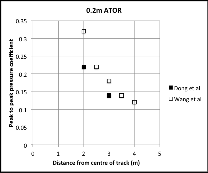
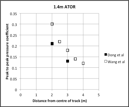
Figure 1 Nose pressure transients

Both papers also give data that enables the peak of the dimensionless nose velocity transient to be determined. Similar data can be obtained from the work of Chen et al (2019a) who investigated the effects of different nose lengths on an idealized high-speed train model. The results are shown in figure 2 for the heights of 0.2m and 1.4m above the top of rail. The data from Chen et al is for a 7.5m nose length. Although this parameter is not tabulated in TAFA, figure 5.2 gives a value of 0.08 at 0.2m above the top of rail, which is consistent the data from the more recent papers. There is again no obvious reason for the difference between the results of Dong et al and Wang et al. The data for Chen et al for a 7.5m nose is close to that of Wang et al at 0.10. For the 5m and 10m nose lengths the values are 0.12 and 0.09.

• 

• 

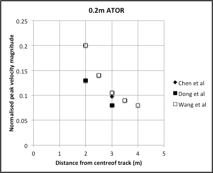
Figure 2. Nose velocity transients

Boundary layer region

In addition to the three papers mentioned in the last section (Chen et al, 2019a; Dong et al, 2019; and Wang et al, 2019), the papers by Li et al (2019) and Wang et al (2018) also give information on the nature of the flow in the boundary layer region along the train side and roof. Li et al (2019) considered the effect of the coupling between two units, comparing the results found for a single 6 coach unit, and those for two coupled three-coach units, both with CRH2 geometry.  Wang et al (2018) used a two-coach model of a more generic high-speed train shape to study the effects of bogies on the flow.  All five papers gave slipstream velocity time histories that were in principle directly comparable, and could also be compared with the full-scale data for high-speed trains in TAFA chapter 5.  The results are plotted in figure 3, with the normalised velocity values being given at the centre of each coach.  The accuracy for the data from the published papers is not high, as I have taken the information from small-scale figures, but it should nonetheless suffice.  Specifically the following sets of data are shown on the graph.

• Chen et al (2019a) – 7.5m nose length
• Dong et al (2019) – Complex bogie
• Li et al (2019) – Single unit
• Wang et al (2018) – Full model
• Wang et al (2019) – No bogie fairings

In general it seems that the slipstream velocities around the CFD models increase much quicker along the train than for the full-scale data, and thus there is much more rapid boundary layer growth in the CFD calculations. There is much scatter however, and some of this growth may be due to the specific model configuration used. For example the Wang et al (2019) data was for the case with no bogie fairings, which might be expected to lead to a rapidly growing boundary layer. That being said, one would actually expect a more rapidly growing boundary layer at model scale than at full scale for trains such as those considered here. For smooth high speed trains, where the analogy with a flat plate boundary layer is appropriate, the ratio of boundary layer thickness to distance from the nose of the train can be expected, very broadly, to be proportional to (Reynolds number based)^-0.2. For a model scale of 1/8 and roughly full scale train speeds, which is the case for most of the calculations considered here, this suggests that at any point on the train, the scaled up boundary layer thickness for the computations should be about 1.5 times the actual full scale size, all other things being equal. For trains with blunter noses, or for freight trains, the size of the boundary layer will be more influenced by local separations and model scale and full-scale values should be more consistent. 

Figure 3. Normalised velocity at 3m from COT and 0.2m above TOR

The growth of the boundary layer has been measured by Chen et al (2019a) in terms of the classic boundary layer parameters of displacement and momentum thickness and form parameter.  His results for the displacement thickness on the side of the train are shown in figure 4 below for both the trackside and the platform cases, and also on the roof of the train. For the train side case, the boundary layer thicknesses from full-scale measurements of the ICE1 are also shown (from TAFA figure 5.12). These can be seen to be somewhat above those of Chen et al (2019a) which is perhaps not surprising as the blunt nosed ICE1 will cause a significant boundary layer thickening near the front of the train.  For both the side and the roof results of Chen the form parameter is around 1.25 to 1.3, somewhat nearer to the classical boundary layer value than the ICE1 values of 1.15.

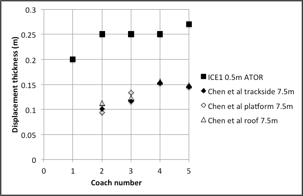
Figure 4 Boundary layer displacement thickness along side of train and roof

Figure 5 again shows the data for Chen et al (2019a) for the train roof, but this time showing the momentum thickness in order to enable a comparison to be made with a comparison with the results of Li et al (2019). The results can be seen to be similar if not identical. 

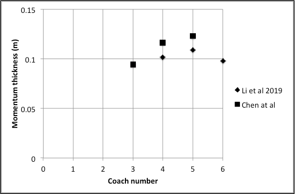
Figure 5 Boundary layer momentum thickness along the roof of the train

In terms of overall boundary layer thickness, Gao et al (2019) and Niu et al (2018b) show contour plots around the train section. The figures shown are too small to take meaningful numbers from, but do indicate the thickening of the boundary layer close to the bogie region, and a slight thinning over the roof of the train. Wang et al (2019) provide rather more information of boundary layer thickness, and the development of the boundary layer down the side of their models is shown in figure 6, in terms of bogie position. These values are consistent with the displacement and momentum thicknesses shown above, being about an order of magnitude greater than the displacement and momentum thicknesses. 

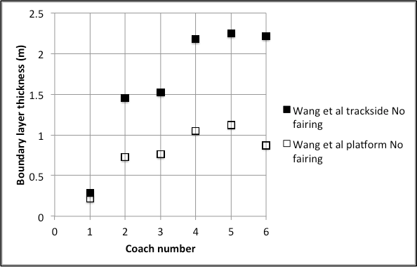
Figure 6 Boundary layer thickness along the side of the train

Wang et al (2019) also give data for the velocity profiles at the side of the train (figure 7). These show the boundary layer extending to 3 to 4.4m from COT, which whilst broadly consistent with the various full-scale data sets in TAFA (figure 5.11), are perhaps somewhat thicker than the full scale results given there.

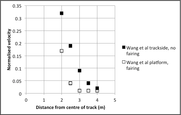
Figure 7 Boundary layer velocity profiles

Finally the individual datasets in some of the papers give useful information of the effect of different train geometries. These are summarised in table 2, which shows the normalised slipstream velocities at 3m from the centre of the track and 0.2m above TOR for the last coach of the train for Chen et al (2019a) (different nose lengths); Li et al (2019) for single and double units; and Wang et al (2019) for bogie fairings. The most noticeable effect is that of the gap between the units in double unit formations. 

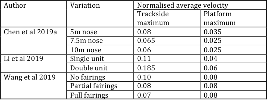
Table 2. Effect of train modifications on normalised velocity (3m from COT, 0.2m above TOR at the centre of the last coach).

Underbody region

Perhaps the most significant paper to consider the flow beneath trains was that of Paz et al (2019) who looked at a novel method of specifying ground conditions that was much more realistic than current methodologies. This involved the scanning of the ballast and sleeper profiles of real track, with all the inherent irregularities and using this as the bottom boundary condition in CFD simulations. They showed that this methodology produced velocity profiles under long trains that conformed well with full-scale experiments, and that results in much more turbulent and chaotic flows than conventional ground simulations. This has obvious implications for the movement of ballast beneath trains. It seems to me that this paper sets the standard for proper ground simulations beneath trains in the future

A number of other papers looked at specific issues to do with the flow underneath the train, but it is difficult to draw any general conclusions from them, partly because they were addressing very localized effects and partly because they in general used short trains where the flows beneath the trains were not fully developed – for example Dong et al (2019) used a 2 car model when investigating different ground simulations; Gao et al (2019) used a three car model to look at bogie effects on the wake flow; Liu et al (2018) used a 1.5 car model to investigate snow accumulation on bogies; and Wang et al (2019) used a 3 car train to investigate the effect of bogie fairings. Whilst all these results are interesting in their own right, their application is very specific to the cases considered.  

Wake

A number of authors considered the wake flow of high-speed trains in some detail, looking at the effect of various geometric changes on the nature of the wake. In all cases the broad structure of the wake was similar to that found by many investigations in the past – a pair of counter-rotating longitudinal vortices. The investigations came to a number of conclusions as to the effect of geometric variations on the strength of this vortex pair as follows. 

• Chen et al (2019a) found that the flow pattern for the shortest of the three train noses they used (5m) created a different wake topology to that with the 7.5m and 10m noses, and higher slipstream velocities. 
• Gao et al (2019) showed that the precise position of the rear bogies had a noticeable, if not major effect upon wake topology. 
• Li et al (2019) looked at the different wakes for single and multiple unit trains, They found that the wakes were similar in the two cases, but that for the double unit was more unsteady, reflecting the greater unsteadiness in the separating boundary layer at the end of the train due to the inter-unit gap. Overall they suggested however that the vortex pattern was dominated by the separation from underbody structures.
• Wang et al (2018) showed that the presence of bogies on train models enhanced the unsteadiness of the flow. However the same dominant wake frequencies appeared with and without bogies, suggesting that whilst the vortex pattern results from the separated shear layer from the train, and has a certain fundamental unsteadiness, this unsteadiness is enhanced by the turbulence from the underbody flow
• Wang et al (201), showed, unsurprisingly, that large fairings decrease scale and intensity of wake flow.

Overall these results suggest that the counter-rotating flow behind a high speed train is basically formed from the separating shear layers from the train side and roof boundary layers, but can be significantly modified by high levels of turbulence in the underbody flow. Here a word of caution is appropriate. As noted above, the underbody flow is the most difficult to simulate and really requires long trains and a sophisticated ground simulation, neither of which is usually the case in most CFD calculations. Thus the calculated effects of underbody flow or geometric changes on the wake structure must only be regarded as illustrative. There is a danger of reading too much into the various CFD results with regard to the wake structure. In addition it has been pointed out in TAFA that wake flows are quite sensitive to even small cross winds. Such winds will have length scales of the same approximate size as the vortex scale and it can be expected that in reality the general vortex flow pattern will be significantly distorted by such effects. Care should thus be taken so as not to overanalyze CFD models of wake flows. 

These points having been made, it is possible to extract from the various papers values of the average maximum wake flow velocity, and the TSI gust velocity. These values are shown in tables 3 and 4 below for the trackside TSI position 3m from COR and 0.2 ATOR for both single and double units, together with data from TAFA. Very broadly the ensemble mean maximum peak for the CRH2 tests is consistent with the published data, as are the TSI gust measurements, for both single and double units. The ensemble mean maximum for the generic high speed trains than  are however lower than the published values.

If one accepts that the wake structure is largely determined by the nature of the separating boundary layer at the end of the train, the fact that the CRH2 results are similar to the full scale results is perhaps a little surprising, in that the train boundary layers seem to grow more rapidly at model scale than at full scale (see above). It may be that this effect is compensated for by two effects; firstly that the model scale trains are shorter than the full scale trains, and thus the boundary layer at the end of the model scale trains will have a scaled thickness similar to that at full scale; and secondly it may be that the wake flow is not overly sensitive to the precise boundary layer characteristics at the end of the train. Nonetheless it does suggest some caution is required in the interpretation of slipstream measurements from reduced scale physical or computational tests for high speed, relatively smooth trains. 

Table 3 Wake velocities for single units

Table 4 Wake velocities for double units

Crosswind

Of the papers reviewed, four of them looked at specific crosswind effects

• Chen et al (2019b) investigated the effect of nose length on cross wind pressures on the train. These were found to be small except around the nose and the tail.  
• Guo et al (2019) compared the crosswind behavior of single and double units in terms of cross wind forces and wake characteristics. 
• Li et al (2018) looked at the effect of crosswinds on pantograph forces, and also presented some useful calculations of train roof boundary layers in crosswinds. 
• Niu et al (2018a) considered the effects of wind breaks on cross wind forces and wake characteristics.

All the calculations presented in the above papers give details of the inclined vortex wake behind the trains in low yaw angle crosswind conditions, and analyse these wakes in some depth. Now, none of the simulations attempted to reproduce atmospheric turbulence, so they are all unrealistic in this regard. The length scales of atmospheric turbulence near the ground are of the same order of size as the trains and the inclined vortices in the train wake. Thus in reality train wakes will be very disrupted by atmospheric turbulence and the detailed patterns observed in the CFD results will not occur. This suggests that to carry out a detailed analysis of the train wake is to over interpret the results. 

Thus in what follows, we do not look at the detailed results in these papers, but rather the results for global force coefficients that can be used to expand the existing database of information on crosswind forces on trains. Force coefficient data is given in Guo et al (2019), Li et al (2018) and Niu et al (2018a). Side force and lift force coefficients are set out in tables 5 to 7, with the reference area taken as 10m²in the conventional way. Two major points arise from these tables.

• There is little difference between single and multiple unit crosswind forces, except for the cars near the junction between the two sets.
• The windbreak calculations suggest there can actually be significant negative side forces on trains behind wind breaks under some circumstances.

Table 5. Force coefficient data from Guo et al (10 degrees yaw)

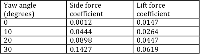
Table 6 Pantograph force coefficients from Li et al (2018)

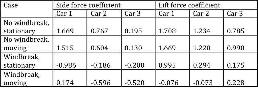
Table 7 Train force coefficients from Niu et al (2018a) (15 degrees yaw, Zero porosity windbreak)