Pollutants, pathogens and public transport – ventilation, dispersion and dose

Preamble

The ventilation of buses and trains has come to be of some significance to the travelling public in recent years for a number of reasons. On the one hand, such vehicles can travel through highly polluted environments, such as urban highways or railway tunnels, with high levels of the oxides of nitrogen, carbon monoxide, hydrocarbons and particulate matter that can be drawn into the passenger compartments with potentially both short- and long-term health effects on passengers. On the other, the covid-19 pandemic has raised very significant concerns about the aerosol spread of pathogens within the enclosed spaces of trains and buses. There is a basic dichotomy here – to minimise the intake of external pollutants into vehicles, the intake of external air needs to be kept low, whilst to keep pathogen risk low, then high levels of air exchange between the outside environment and the internal space are desirable. This post addresses this issue by developing a common analytical framework for pollutant and pathogen dispersion in public transport vehicles, and then utilises this framework to investigate specific scenarios, with a range of different ventilation strategies.

Analysis

The basic method of analysis is to use the principle conservation of mass of pollutant or pathogen into and out of the cabin space. In words this can be written as follows.

Rate of change of mass of species inside the vehicle = inlet mass flow rate of species + mass generation rate of species within the vehicle – outlet mass flow rate of species– mass flow rate of species removed through cleaning, deposition on surfaces or decay.

This results in the equation shown in Box 1 below, which relates the concentration in the cabin to the external concentrations, the characteristics of the ventilation system and the characteristics of the pollutant or pathogen. The basic assumption that is made is of full mixing of the pollutant or pathogen in the cabin. The pdf gives full details of the derivation of this equation, and of analytical solutions for certain simple cases. It is sufficient to note here however that this is a very simple first order differential equation that can be easily solved for any time variation of external concentrations of pollutant generation by simple time stepping methods. For gaseous pollutants, the rate of deposition and the decay rate are both zero which leads to a degree of simplification.

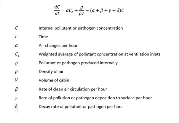
Box 1. The concentration equation

The pdf also goes on to consider the pollutant or pathogen dose that passengers would be subjected to – essentially the integration of concentration of time history – and then uses this in a simple model of pathogen infection. This results in the infection equation shown in Box 2. Essentially it can be seen that the infection risk is proportional to the average concentration in the cabin and to journey length.

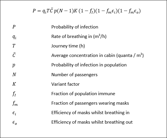
Box 2. Infection equation

The main issue with this infection model is that it assumes complete mixing of the pathogen throughout the cabin space and does not take account of the elevated concentrations around an infected individual. A possible way to deal with this is set out in the pdf. Further work is required in this area.

Ventilation types

The concentration and infection equations in Boxes 1 and 2 do not differentiate between the nature of the ventilation system on public transport vehicles. Essentially there are five types of ventilation.

• Mechanical ventilation by HVAC systems
• Ventilation through open windows
• Ventilation through open doors
• Ventilation by a through flow from leakage at the front and back of the vehicle (for buses only)
• Ventilation due to internal and external pressure difference across the envelope.

Simple formulae for the air exchange rates per hour have been derived and are shown in Box 3 below. By substituting typical parameter values the air exchange rates are of the order of 5 to 10 air changes per hour for the first four ventilation types, but only 0.1 for the last. Thus ventilation due to envelope leakage will not be considered further here, although it is of importance when considering pressure transients experienced by passengers in trains.

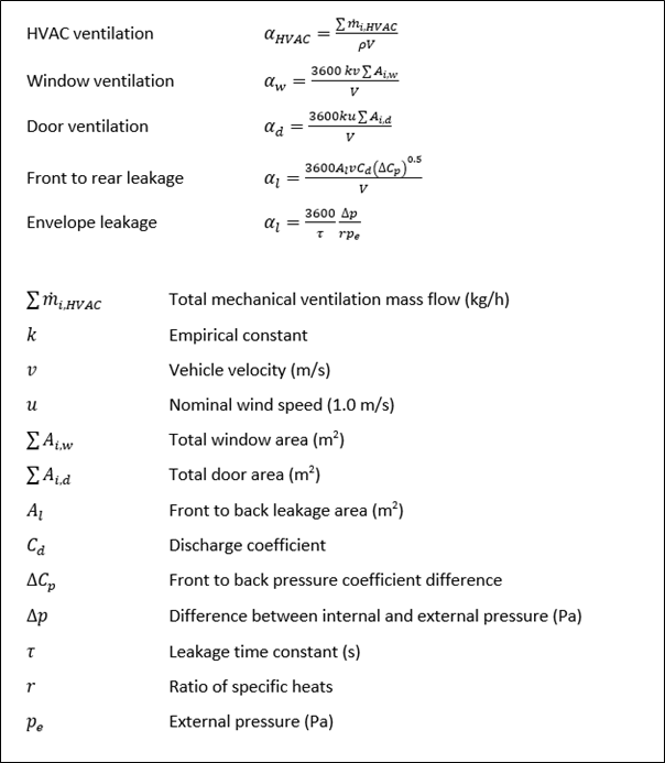
Box 3. Ventilation types

Scenario modelling

In what follows, we present the results of a simple scenario analysis that investigates the application of the above analysis for different types of vehicle with a range different ventilation systems, running through different transport environments. We consider the following vehicle and ventilation types.

• An air-conditioned diesel train, with controllable HVAC systems.
• A window and door ventilated diesel train.
• A bus ventilated by windows, doors, and externally pressure generated leakage.

Two journey environments are considered.

• For the trains, a one-hour commuter journey as shown in figure 1, beginning in an inner-city enclosed station, running through an urban area with two stations and two tunnels, and then through a rural area with three stations (figure 1).
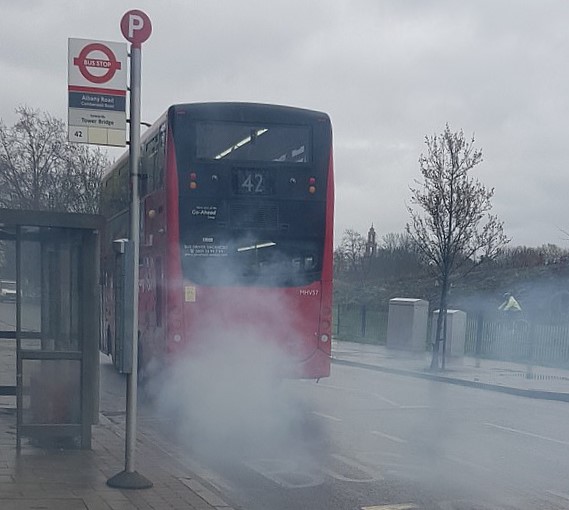
• For buses, a one-hour commuter journey, with regular stops, through city centre, suburban and rural environments (figure 2).

Results are presented for the following scenarios.

• Scenario 1. Air-conditioned train on the rail route, with HVACs operating at full capacity throughout.
• Scenario 2. As scenario 1, but with the HVACs turned to low flow rates in tunnels and enclosed stations, where there are high levels of pollutants.
• Scenario 3. Window ventilated train on rail route with windows open throughout and doors opened at stations.
• Scenario 4. As scenario 3, but with windows closed.
• Scenario 5. Window, door and leakage ventilated bus on bus route with windows open throughout and doors opened at bus stops.
• Scenario 6. As scenario 5, but with windows closed.

Details of the different environments and scenarios are given in tables 1 and 2.  Realistic, if somewhat arbitrary levels of environmental and exhaust pollutants are specified for the different environments – high concentrations in cities and enclosed railway and bus stations and lower concentrations in rural areas. The air exchange rates from different mechanisms are also specified, with the values calculated from the equations in Box 3. Note that, in any development of this methodology, more detailed models of the exhaust emissions could be used that relate concentrations at the HVAC systems and window openings to concentrations at the stack, which would allow more complex speed profiles to be investigated, with acceleration and deceleration phases.

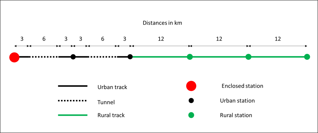
Figure 1. The rail route

Figure 2. The bus route

Table 1. The rail scenarios

Table 2. The bus scenarios

The results of the analysis are shown in figures 3 and 4 below for the train and bus scenarios respectively. Both figures show time histories of concentrations for NO2, PM2.5, CO2 and Covid-19, together with the external concentrations of the pollutants.

For Scenario 1, with constant air conditioning, all species tend to an equilibrium value that is the external value in the case of NO2 and PM2.5, slightly higher than the external value for CO2 due to the internal generation and a value fixed by the emission rate for Covid 19.

For Scenario 2, with low levels of ventilation in the enclosed station and in the tunnels, NO2 and PM2.5 values are lower than scenario 1 at the start of the journey where the lower ventilation rates are used, but CO2 and Covd-19 concentrations are considerably elevated. When the ventilation rates are increased in the second half of the journey all concentrations approach those of Scenario 1.

The concentration values for scenario 3, with open windows, match those of Scenario 1 quite closely as the specified ventilation rates are similar. However, for Scenario 4, with windows shut and only door ventilation at stations, such as might be the case in inclement weather, the situation is very different, with steadily falling levels of NO2 and PM2.5, but significantly higher values of CO2 and Covid-19. The latter clearly show the effect of door openings at stations.

• 

• 

• 

• 

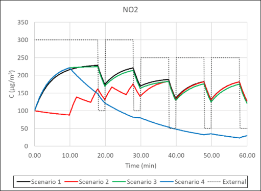
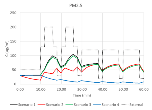
Figure 3. The train scenario results

Now consider the bus scenarios in figure 4. For both Scenario 5 with open windows and doors, and Scenario 6 with closed windows and open doors, the NO2 and PM2.5 values tend towards the ambient concentrations and thus fall throughout the journey as the air becomes cleaner in rural areas. The internally generated CO2 and Covid-19 concentrations for CO2 and Covid-19 are however very much higher for Scenario 6 than for Scenario 5.

• 

• 

• 

• 

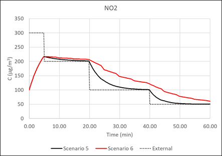
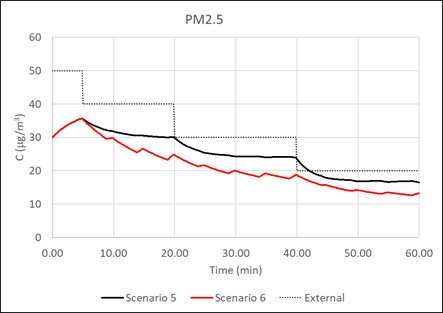
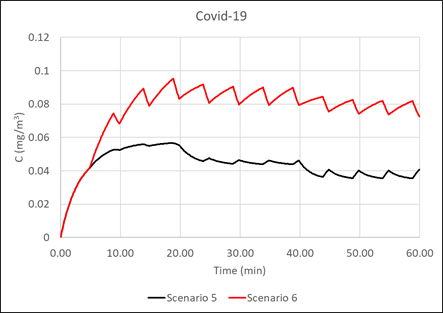
Figure 5. The bus scenarios

The average values of concentration for all the scenarios is given in Table 3. The dose and, for Covid-19, the infection probability, are proportional to these concentrations. For NO2 and PM10 the average concentrations reflect the average external concentrations, and, with the exception of Scenario 4, where there is low air exchange with the external environment for part of the journey. The average concentrations for CO2 and Covid-19 for the less ventilated Scenarios 4 and 6 are significantly higher than the other. For Covid-19, the effect of closing windows on window ventilated trains and buses raises the concentrations, and thus the infection probabilities, by 60% and 76% respectively.

Table 3. Average concentrations

Closing comments

The major strength of the methodology described above is its ability, in a simple and straightforward way, to model pollutant and pathogen concentrations for complete journeys, and to investigate the efficacy of various operational and design changes on these concentrations. It could thus be used, for example, to develop HVAC operational strategies for a range of different journey types. That being said, there is much more that needs to be done – for example linking the methodology with calculations of exhaust dispersion around vehicles, with models of particulate resuspension or with models of wind speed and direction variability. It has also been pointed out above that the main limitation of the infection model is the assumption of complete mixing. The full paper sets out a possible way forward that might overcome this. Nonetheless the model has the potential to be of some utility to public transport operators in their consideration of pollutant and pathogen concentrations and dispersion within their vehicles.