Nomenclature
This post addresses the issue of the use of what has become known as the “Chinese Hat” gust model. The use of this title has become increasingly problematic over recent years for obvious reasons, and I will no longer use it, but will instead refer to the “CEN extreme gust model” in what follows.
The CEN extreme gust model
In a number of situations in wind engineering, some sort of deterministic (as opposed to stochastic) gust model is required in order to determine structural response. One such case is in the determination of the risk of overturning of road or rail vehicles in high winds. A methodology of this type is set out in CEN (2018), where an extreme gust model is described. This model was originally developed in wind loading studies for wind turbines as a time dependent gust to be applied to calculate wind turbine loading at one fixed location (Bierbooms and Cheng, 2002). As such, it is perfectly adequate and a good representation of an average extreme gust in high wind conditions. In the methodology of CEN however, it is re-interpreted as a stationary spatially varying gust. This must be regarded as a very significant assumption for which, in my view, there is little justification. Nonetheless the formulation has proved useful practically and we begin by considering it in a little more detail.
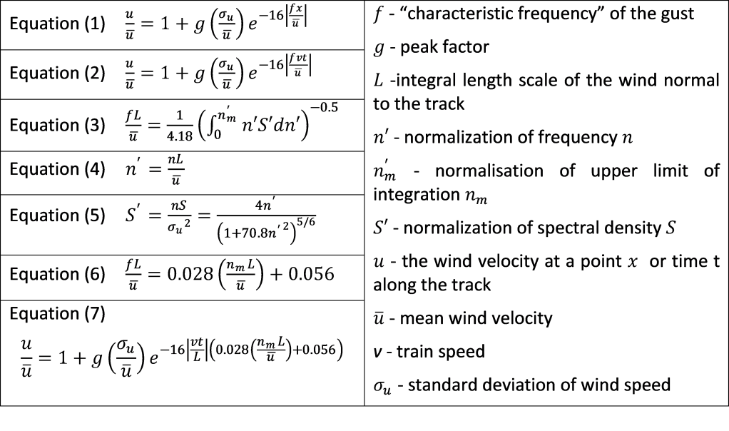
For a wind normal to the track, the extreme gust formulation is given by equation (1) on Box 1. Note that the “characteristic frequency” of the gust is calculated from standard wind engineering methods for temporally, rather than spatially, varying gusts. Equation (1) is a generalised form of that given in CEN (2018) to remove some of the constants that tie the expression to a particular location and topography through specific values of peak factor and the turbulence intensity (the ratio of the standard deviation to the mean velocity). The time dependence is recovered through the passage of the train passing through this gust at a speed v = xt to give equation (2). It can be seen that the gust thus has a maximum value of (1+ peak factor x turbulence intensity) when t = 0 and decreases to unity for small and large times. It is symmetrical about t = 0. The velocity relative to the train is then found by the vector addition of this gust velocity with the vehicle velocity to give a time varying value.
To enable the gust profile to be specified, the characteristic frequency f is required. This is specified in equations (3) to (5). These equations are again in a more generalized form than given in CEN (2018), where a value of the upper limit of integration is fixed at 1 Hz, together with an implicit value of the turbulence length scale of around 75m. The genesis of the 4.18 factor is however not clear to me. Equation (3) shows that the calculation of the characteristic frequency is thus based on the calculation of the zero-crossing rate of temporal fluctuations through the use of the velocity spectrum. Again, note that these parameters describe a time varying rather than a spatially varying velocity, and their use is not formally consistent with a spatially varying gust. From equations (3) to (5), it can be seen that the normalized characteristic frequency is a function of the normalized upper limit of integration. A numerical solution of these equations was carried out and the following empirical line fitted to the results for a value of the latter greater than 1.5 (which is the realistic range) – equation (6). From equations (2) and (6) we thus obtain equation (7). Although the overall methodology cannot be regarded as wholly sound, equation (7) does (in principal) significantly simplify its use and also allows the implicit wind parameters in the method to be explicitly defined.
Is there a better methodology?
It can be seen from the above that the CEN methodology thus does not fully describe a typical gust as seen by a moving train, which would vary both spatially and temporally, and can at best be regarded as an approximation, although its practical utility must be acknowledged. Ideally, if such an approach is to be used, a gust that varies both in space and time is really required. Such a gust was used in the SNCF route assessment method of Cleon and Jourdain (2001), where the shape of the gust is appropriately described as a rugby ball. This method was however for very specific wind characteristics and does not seem to have found widespread use. Thus in this post, we investigate the possibility of developing a spatially and temporally varying gust, that can be expressed in a simple form (ideally similar to equation (2)) for practical use.
Towards a new model
In this section we will draw on experimental results for extreme gust characteristics in both temporal and spatial terms to construct a simple, if empirical model, that fulfills the function of the CEN (2018) model without the theoretical drawbacks.
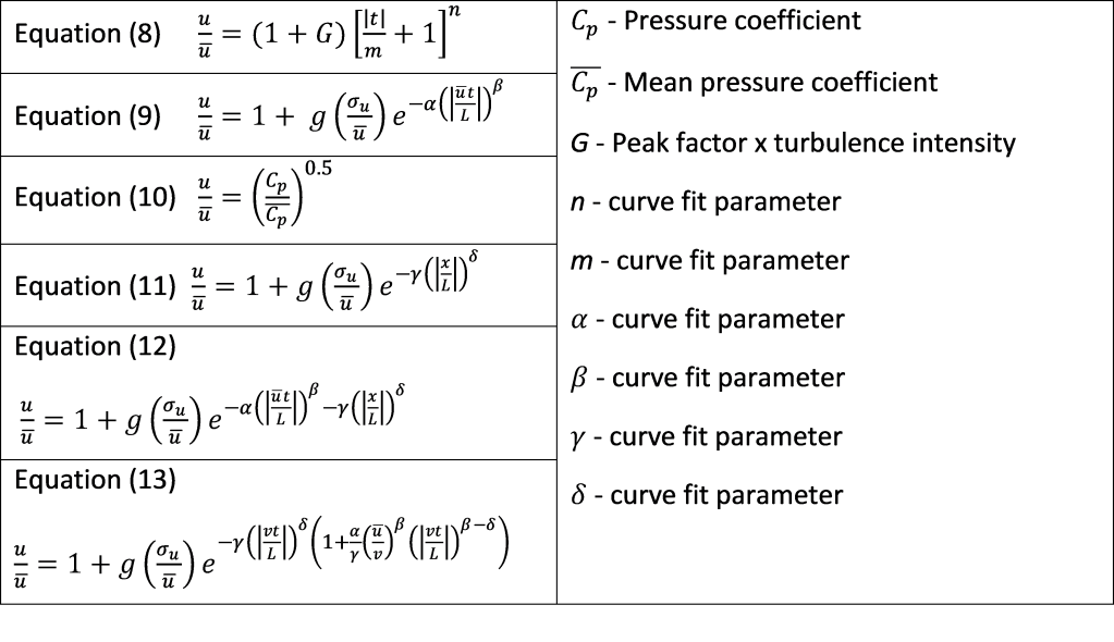
We consider first the full-scale experimental data analysed by Sterling et al (2006) which used conditional sampling to determine the average 99.5th percentile gust profile for four anemometers on a vertical mast with heights between 1m and 10m. These results thus give the time variation in gust speed as the gust passes the anemometers. They showed that the gust profiles could be well approximated by the formula shown in equation (8) (Box 2). The parameter G in this equation is the equivalent of the peak factor multiplied by the turbulence intensity in equation (2) and for these measurements was 0.786. n was -0.096, and the value of m depended upon whether t was greater or less than zero. For t < 0, i.e. on the rising limb, m was 0.1, whilst for t > 0, on the falling limb, m was 0.2. The gust shape was thus asymmetric with a maximum at t = 0. This curve was a good fit to all the gust profiles throughout the height range. In what follows we will use a rather different curve fit expression to the same data, more consistent with that used in CEN (2018) – equation (9). It was found that the best fit value of b was equal to 0.5 for all t, whilst the best fit values of a were 0.49 for the rising gust and 0.37 for the falling gust. This expression thus describes the temporal variation of wind speed as a gust passes through the measuring point
To describe the lateral spatial variation of the gust profile, we use the data of Baker (2001) who presents conditionally sampled peak events for pressure coefficients along a 2m high horizontal wall. This data allows the lateral extent of the gusts to be determined, from the variation of the time varying pressure coefficient divided by the mean value of the coefficient and then assuming that the gust velocity variation can be found from equation (10). The spatial variations of velocity were then fitted by a curve of the form of equation (11). g was found to be 6.16 and d was found to be 0.7.
On the basis of the above expressions one can thus write the expression of equation (12), which describes the variation of the gust velocity in both space and time. The movement of the train through the gust can again be allowed for by letting x = vt (equation (13)).
Model comparison
Box 3 sets out the formulations of the CEN extreme gust model and the model derived here. In some ways they are similar in form, with an exponential formula that is primarily a function of normalized time. Whilst the CEN model is symmetric around t = 0, the new model has a degree of asymmetry because of the different values of the curve fit parameters for t < 0 and t > 0. However an examination of the new model suggest that the asymmetric term may be small, and thus Box 3 also shows an approximate version of the new model where this term is neglected.
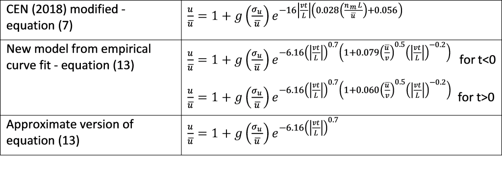
Figure 1 shows a comparison of these three models for the following parameter values – peak factor = 3.0; turbulence intensity = 0.25; train speed = 75m/s; mean wind speed = 25m/s; turbulence length scale = 75m, upper frequency of integration = 1.0Hz. It can be all three models are similar in form, showing a sharp peak at t = 0. The full and approximate forms of the new model are almost indistinguishable, showing that the approximation suggested above is valid. The main difference is that the CEN model has a much greater spread in time than the new model. This difference persists whatever input parameters are chosen.
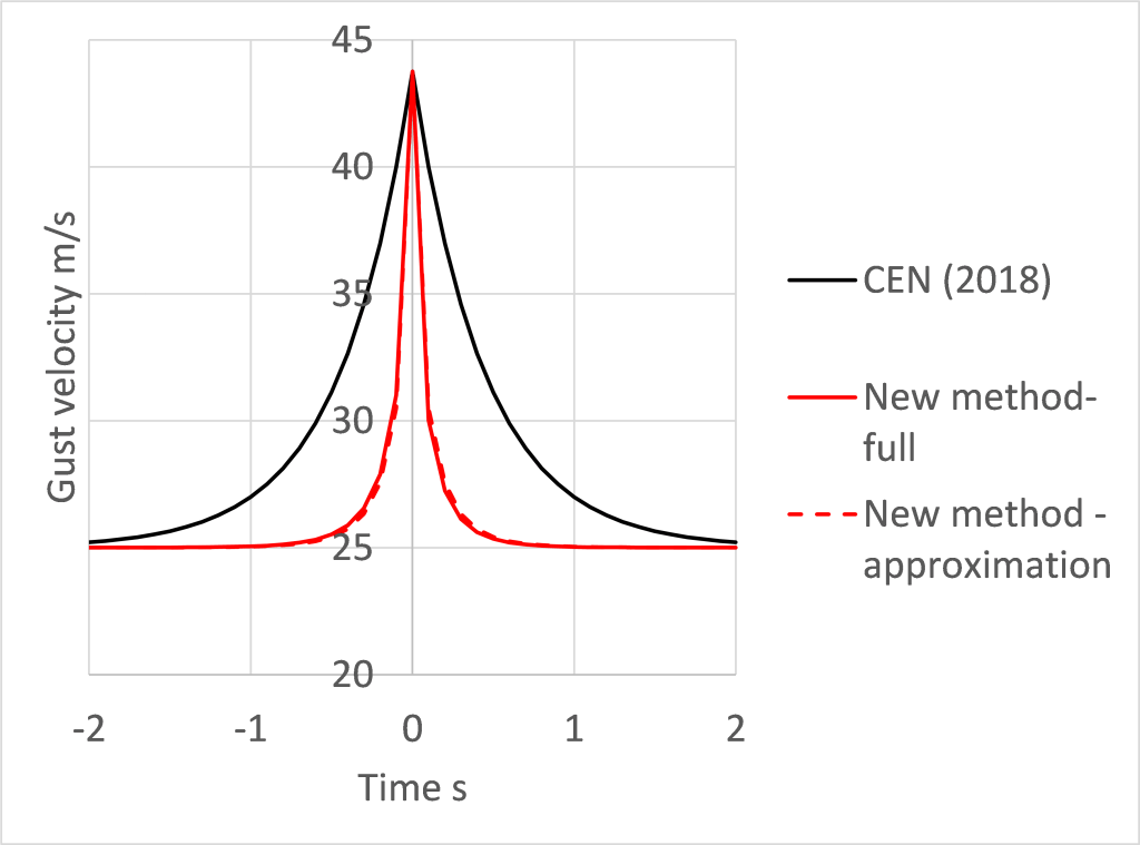
At this point it is necessary to consider again the genesis of the models – the CEN model resulted from an application of a time varying gust model as a spatially varying gust model, whilst the new model was developed based on measured temporal and spatial gust values. As such, I would expect the latter to be more accurate. The broad spread of the CEN gust may result from an application of the time varying along wind statistics to a cross wind spatial gust. Since it is known that that longitudinal integral scale is several times larger than the lateral integral scale, this would result in a wider spread of the gust than would be realistic. This is to some extent confirmed by the period of the two gusts – around 2s for the CEN gust and around 0.8s for the new model. For a train speed of 75m/s, this corresponds to gust widths of 150m and 60m – roughly approximating to the expected the longitudinal and lateral turbulence integral scales.
Concluding remarks
In this post I have looked again at the CEN extreme gust method and raised concerns about its fundamental assumptions. I have also developed an equivalent, but perhaps more rigorous, methodology based on experimental data for wind conditions at ground level. This strongly suggests that the CEN gusts are spatially larger than they should be, which suggests its long term use should be reviewed. However, when used to compare the crosswind behaviour of individual trains, rather than in an absolute sense, it is probably quite adequate.
References
Baker C J, 2001, Unsteady wind loading on a wall, Wind and Structures 4, 5, 413-440. http://dx.doi.org/10.12989/was.2001.4.5.413
Bierbooms, W., Cheng, P.-W., 2002. Stochastic gust model for design calculations of wind turbines. Journal of Wind Engineering and Industrial Aerodynamics 90 (11), 1237e1251. https://doi.org/10.1016/S0167-6105(02)00255-6.
CEN, 2018. Railway Applications d Aerodynamics d Part 6: Requirements and Test Procedures for Cross Wind Assessment. EN 14067-6:2018.
Cleon, L., Jourdain, A., 2001. Protection of line LN5 against cross winds. In: World Congress on Rail Research, Köln, Germany.
Sterling M, Baker C, Quinn A, Hoxey R, Richards P, 2006, An investigation of the wind statistics and extreme gust events at a rural site, Wind and Structures 9, 3, 193-216, http://dx.doi.org/10.12989/was.2006.9.3.193

One thought on “Modelling of extreme wind gusts”