Preamble

In the recently published book “Come wind, come weather” (Lichfield Press, 2021), Trevor James draws attention to the Midland Tornado of 1545 which caused very considerable damage along a very long storm track in Derbyshire. A description of the damage from that time is given in the Derbyshire edition of the Magna Britannia in 1817 and is reproduced below. In this short post, the nature of the storm will first be discussed and then we will make some estimates of the windspeeds that occurred, using modern damage scales. I will then address the question as to whether the event was actually a tornado, or some other type of wind storm.

The event

From the Magna Britannia.

” At Darbie the 25th daye of June 1545.

“Welbeloved sonne I recomend me unto you, gevyng you Godds blessyng & myne. Son this is to sertifie you of soche straunge newes, as that.hath of late chauns,ed in thes p’ties; that is to wytt, apon Satterday last past, being the 20th daye of this moneth, on Say’te Albons day, we had in thes p’tyes great tempest. … wether, about xi of the clok before none: & in the same tempest, The dev[ill] as we do suppose beganne in Nedewood, wch is ix myles from Da[rbie]; & there he caste downe a great substance of wood; & pulled up by the rotts: & from thens he came to Enwalle [Etwall] wher at one Mre Powret [Porte] dothe dwell, & he pulled downe ij great elmes, that there was a dossyn or xvj loode apon a piese of them; & went to the churche & pullyd up the leade, & flonge it apon a great elme that stondyth a payer of butt lenghthes from the churche, &. … it hangyd apon the bowys lyke stremars; & afte. …….. tourned. …… & the grounsells upwards & some layd bye apon. ….. heape &. ……. that was apon viij bayes long he set it a…….. gge & the. …… ro[ots] sett upwards; & he hathein the same towne lefte not past iiij or v housses hole. And from thence he came a myle a this syde, & there grewe opon Ix or iiijxx wyllowes, & apon xij or xvi he hathe brokyn in the mydds, & they were as great as a mans body: & so he lefte them lyke a yard and a half hye: And from thence he went to Langley, wch is lyke iiij myles from Darby, & there he hath pullyd downe a great p’te of the churche, & rowled up the leade & lefte it lyeing, & so went to Syr Wyllam Bassetts place in the same [towne] & all so rente it, & so pullyd a great parte of it downe wth his. …..& the wood that growethe abowte his place, & in his parke he pulled downe his pale & dryve out his deare, & pulled downe his woods, & so[me] broken in the mydds that was xvj or xx loode of wood of some one tre. And after that he went into the towne to Awstens housse of Potts & hath slayne his sonne & his ayer, & perused all the hole towne, that he hath left not past ij hole howsses in the same towne. And from thence he went to Wy’dley lane, & there a nourse satt wt ij chylderen uppon her lappe before the fyre, & there he flonge downe the sayde howse, & the woman fell forwards ap[on the] yongechyl[dren] afore the fyre, & a piese of ty’ber fell apon her. …… & so killed [her] but the chylderen were savyd, & no more hurte, [and none] of the house left standyng but the chymney, & there as the house stode, he flange a great tre, that there is viij or x lood of wood apon it. And from thence he went to Belyer [Belper] & there he hath pullyd & rent apon xl housses; & from thence he wente to Belyer [Belper] wood & he hathe pullyd downe a wonderous thyng of wood & kylled many bease; & from thens to Brege [Heage] & there hath he pulled downe the chappyl & the moste parte of the towne; & from thens to WynfeldmaJ that is the Erie of Shrowseberys [Wingfield Park], & in the parke he pulled him downe a lytell…… & from thens to Manfyld [Mansfield] in Shrewood & there I am sure he hath done [no] good, & as it is sayd he hathe donne moche hurte in Chesshire &….. shire. And as the noyse goeth of the people ther felle in some places hayle stons as great as a mans fyste, & some of them had prynts apon them lyke faces. This is trewe & no fables, there is moche more hurte done besyds, that were to moche to wryte, by the reporte of them that have sene it; and thus fare you well.”

James is persuaded that the account is genuine, not least by the mention of the damage to the chapel at Heage. The church at Heage was indeed officially a chapel (dependent upon another church) at the time and there are records elsewhere that indicate it was rebuilt after the storm. James quotes a further source (Warkworth’s Chronicle) which again suggests strong winds in Cheshire and Lancashire on that day.

The personification of the event as the “devil” is of interest and may reflect both the belief that such events were demonically rather than divinely inspired but might also refer to the name of such events – indeed even today small whirlwinds are referred to as dust-devils or something similar.

The description allows the track of the storm to be determined quite accurately, and this is shown on the map of figure below. In all the track where precise damage details are given seems to have been about 40 km long at least.

Wind speeds

On the assumption that we are dealing with an tornado here, rather than another type of windstorm (see below), is it possible to obtain estimates of what the windspeeds actually were? Tornado windspeeds are usually estimated by inspecting the damage that they cause, and then using a damage classification method to determine the broad range of wind speeds that would cause that damage. Two methods are commonly used – the Enhanced Fujita (EF) scale developed in the US, and the T scale developed by the Tornado Research Association TORRO. Extracts from the damage descriptors are given below.

Enhanced Fujita EF Scale

EF2         49–60m/s      Roofs torn off from well-constructed houses; foundations of frame homes shifted; mobile homes completely destroyed; large trees snapped or uprooted; light-object missiles generated; cars lifted off ground.

EF3         60-74m/s      Entire stories of well-constructed houses destroyed; severe damage to large buildings such as shopping malls; trains overturned; trees debarked; heavy cars lifted off the ground and thrown; structures with weak foundations are badly damaged.

EF4 74-89m/s Well-constructed and whole frame houses completely leveled; some frame homes may be swept away; cars and other large objects thrown and small missiles generated.

TORRO T scale

T4           52 – 61m/s           Motor cars levitated. Mobile homes airborne / destroyed; sheds airborne for considerable distances; entire roofs removed from some houses; roof timbers of stronger brick or stone houses completely exposed; gable ends torn away. Numerous trees uprooted or snapped.

T5          62- 72m/s            Heavy motor vehicles levitated; more serious building damage than for T4, yet house walls usually remaining; the oldest, weakest buildings may collapse completely.

T6           73 – 83m/s          Strongly built houses lose entire roofs and perhaps also a wall; windows broken on skyscrapers, more of the less-strong buildings collapse.

To give some context, the Birmingham Tornado of 2005 (pictured above), one of the strongest in recent years, was classified as a T5 event.

It is immediately clear that these descriptions are very subjective and the classification of damage into a particular class is not straightforward. It is perhaps less clear that each of these scales is to some extent culturally dependent. The EF scale reflects North American building and vehicle types, and the T scale reflects building and vehicle types from the UK in the 1970s when the scale was first produced. Neither reflects building practice in the 1540s and neither were there any cars to be lifted up in that period!  Nonetheless, the description of 1545 can be used within these classifications at least in an approximate way. I would thus classify the 1545 event as borderline EF2 / EF3 or borderline T4/T5. These classifications give a wind speed range around 135 mph or 60 m/s. However,  Neaden, in a study of tornado risk for the HSE, based on the above description, assigns a category of T6 to the event, giving a wind speed of at least 73m/s. This again illustrates the subjectivity of the classification.

The T scale also gives a classification based on path length

T4 2.2 to 4.6km

T5 4.7 to 9.9km

T6 10 to 21km

T7 22 to 46km

On the basis of path length Neaden again gives a T6 classification, although the length as shown in figure 1 suggests a T7 classification. My view would be that the event should properly be categorised as EF2/EF3 or T4/T5 with an unusually long path length but the subjectivity of this assessment must again be emphasised.

Was it a tornado?

The question that then needs to be addressed is whether or not the 1545 event was a tornado or some other storm type – presumably one of the usual extra-tropical cyclones that pass across the UK quite frequently. Even in such storms there are known to be smaller tracks of major damage. In the 1987 storm for example there was a swathe of extreme damage to trees in a arc a few miles wide across the south of England. This was attributed to a high-level jet of wind sweeping down to ground level – a phenomenon know as a “sting jet” because of the scorpion tail-like cloud formation with which such events are often associated. 

The points that suggest the event was a tornado are firstly the existence of a coherent storm track, albeit significantly longer than would normally be the case, and secondly the fact that the event occurred in June, when extra-tropical cyclones are uncommon but tornadoes are. On the other hand, the point that suggest the damage was due to an extra-tropical cyclone is the reference in more than one source to concurrent strong winds in Cheshire and Lancashire. Indeed, wind speeds of 60 m/s have been measured in extra-tropical cyclones in the past – for the 1987 Burns Night storm for example the peak wind speed was somewhere around this value.

Referring again to the work of Neaden, his data indicates that between 1800 and 1985 there were around 10 tornadoes with a classification of T5 or higher in Derbyshire. This indicates that one would occur on average every 20 years or so. One would expect that most of these would have path lengths of a few kilometres and thus the effects would be localised – and in a rural county like Derbyshire not much damage might be recorded.

Now, one might expect that an extra-tropical cyclone with wind speeds of the order of 60m/s would only occur in lowland Britain once every 200 to 300 years – indeed the 1987 storm was assessed as having this return period. Thus they are very rare events indeed.

A comparison of the likelihoods of a T5 tornado and an extra-tropical storm with the same windspeeds thus suggests to me that it is most likely that the 1545 event was indeed a tornado with an EF2 / EF3 or T4/T5 classification, albeit with an unusually long storm track, but also that it was quite possibly embedded in a larger extra-tropical cyclone of some strength. However, as with any other historical phenomenon of this type, absolute certainty as to its cause is of course not possible.

In recent weeks an extraordinary Twitter argument has broken out concerning how much the railway system in the UK and Ireland owes to the capital provided by the slave trade. On the one hand we have Gareth Dennis (@GarethDennis), the author of what will be referred to in what follows as the “Thread”, who argued “that a significant proportion of slave-owner compensation was reinvested into the railways; that Britain’s railways are a direct legacy of slavery and colonialism; and that this legacy is hopelessly under-explored”. On the other hand there was a strong argument from Christian Wolmar (@christianwolmar) that the Thread’s arguments were overstated and not properly evidenced. He has repeated this in a recent edition of RAILmagazine. This post is concerned with trying to establish how much slave owner compensation might have been used for capital investment in the early railway network in the Great Britain and Ireland.

The Thread uses the quite outstanding UCL web site “Legacies of British Slave-ownership” which attempts to chart where the legacies of slave ownership, and in particular the compensation paid to slave-owners following theSlave Compensation Actof 1837, was used in commercial and social ventures.  The Thread takes the data from this web site for those who had both been compensated, and who also invested in the early railway companies, and a simple addition of the sum invested by these individuals in railway companies in Great Britain and Ireland comes to £5,261,768 (a little less than in the Thread, no doubt due to a minor omission somewhere that I can’t locate, but this is of no consequence to what follows). The implication in the Thread is that this sum comes directly from slave compensation and it is argued that this forms a significant proportion of the railway capital in the early years – for example the cumulative capital by 1840 was £30 million, and thus the total invested by the slave owners was around 1/6^thof the total.  

However, all is not as simple as it looks. Firstly, an inspection of the UCL web entries indicates that a few of the identifications of slave owners with railway investors are not totally firm and that there is some doubt about them. Nonetheless these are unlikely to affect the above figure significantly, perhaps reducing it by a few tens of thousands pounds and no correction will be made. Secondly the web site lists a few payments to trustees, usually of minors. It is a moot point as to whether the future railway investment of these trustees in their own right should be included in the sum. Again, this is not a significant issue and no corrections have been made for it. 

A much bigger issue however is that, as I read it, the UCL web site shows the total investment of individuals in the railways, and that is what the figure of £5,261,768 actually refers to. Many of the slave-owners received far less in compensation than they actually invested in the railways – these figures are given on the pages for individuals in the list. So that figure for capital investment, which the Thread uses as the basis for its arguments, is a very significant overestimate of they investments that were made from slave compensation. For example, consider the three individuals who feature in the Thread. The first, John Moss invested £222,470 in railway concerns, but only received £40,353 in slave compensation; Robert Browne invested £577,260 but only received £797 in compensation; and Thomas Dunlop Douglas invested £396,100 having received £15,907 in compensation. One Robert Pulsford is included in the database as investing £291,000 in railways concerns. However his inclusion is as a result of five unsuccessful claims for compensation and he actually received no compensation at all. Similar discrepancies between total investment and compensation sums can be identified for nearly all the major investors, although the amounts invested for the smaller investors were often very similar to the amount of compensation they received. So the figure of £5,261,768 money that found its way into the railways cannot all be from compensation payments. In fact if one limits the amount of investment for each investor to the amount they received in compensation, the figure falls to £1,134,031 i.e. 21.6% of the original figure.  

But even this is without doubt an overestimate, as not all the compensation money would have been invested in the railways. It might be more realistic to say that the proportion of invested compensation should be the same as the proportion of the total investment to the overall wealth of the investor. The UCL site allows an estimate to be made of this for a subset of those named by giving their recorded wealth at death. The median of the ratio of investment to total wealth at death comes to 10% (excluding those individuals who went bankrupt or suffered major financial distress at the end of their lives). I am of course very well aware that this methodology is more than a little suspect! On this basis however the amount of slave-compensation money that was invested in the railways falls to around £110,000.

On the basis of these figures, the actual amount of compensation that became railway capital was between £0.1 million and 1 million. Whether of not this is significant in terms of the overall capital investment (£30 million by 1840) I will let the reader decide.  But it is best to use as accurate a figure as possible in coming to a view.

The Thread has done the community a service by raising the issue of slave-compensation investment on the railways, which should not be ignored, although it needs to be carefully looked at to investigate whether it was significant in comparison to other investment. In future posts, I intend to look at this issue further – both in relation to those who received large compensation sums and made large investments in the railways (not necessarily those mentioned in the Thread); but also in relation to that area of the Black Country about which I have posted regularly – the parish of Kingswinford – where traces of slave-owner investment can indeed be found if one looks carefully. 

In coming to a the definition of the Original Mercia outlined in “The first Mercian Lands”, I included Seisdon Hundred in south Staffordshire within its bounds (figure 1). The reason for doing so was primarily because this area became part of the Mercian Diocese of Lichfield. However there is some rather disparate evidence that at least part of Seisdon hundred was Hwiccan territory at some stage before the formation of the diocese. 

• Topographically, the area is in the catchment of the Smestow and Stour and thus of the Severn itself, as is the case for the other Hwiccan territories. Other parts of Staffordshire are in the Trent catchment.
• There are Domesday linkages between the manors of Tardebigge and Clent in Worcestershire and Kingswinford in Staffordshire – and indeed Clent was for many centuries post-Domesday an island of Staffordshire within Worcestershire.  
• The manors of Kingswinford and Amblecote (in Staffordshire) and Oldswinford (in Worcestershire) were almost certainly once part of the same land unit. 
• The ecclesiastical parish of Oldswinford was split between the manors of Oldswinford in Worcestershire and Amblecote in Staffordshire.
• The large Worcestershire enclave of Dudley has been surrounded by Staffordshire since the Domesday survey.
• The name of the Hundred itself is taken from the village name of Seisdon, which can plausibly be translated as the Hill of the Saxons. This ties in with the now rather dated assumption that the Hwicce represent the northward advance of Saxons up the Severn valley.

Thus a case can be made that the area of Seisdon Hundred was originally Hwiccan territory that was absorbed into the Original Mercia. The reason for this is clear from the map of figure 1 – strategically it is a very important area. The Roman road system centred on Greensforge controls access along the Saltway from Droitwich to the north, access to Shropshire, the borders and Wales, and gives a direct link to Quatford on the Severn, allowing control of river traffic. Three potential roads are shown on the map that are not shown on the larger scale map of figure 8 in the main text – those from Greensforge north east to Wall, from Water Eaton to Metchley and from Metchley to Greensforge. The routes of the first two can be traced in places on the ground (Horovitz, 2005; Bassett, 2001), but the lines shown on the map are purely conjectural. It is however likely that the two routes crossed at Wednesbury. The route between Metchley and Greensforge (Baker, 2013) begins with the Metchley to Water Eaton route but branches from it through the village known as the Portway near Oldbury and then passing though, or to the south of Dudely, to Kingswinford and Greensforge.  Taken together this road network clearly adds to the connectivity of the region and emphasises its strategic importance. 

Figure 1 – Seisdon Hundred

(Red shows boundary of the hundred  – a solid line where it coincides with the county boundary, and a dotted line otherwise; grey shows other county and hundred boundaries; brown shows the pre-1974 county boundary, reflecting the early post-Domesday losses to Shropshire; roads are shown (schematically) in green and rivers in blue).

D Horovitz (2005) “Place names of Staffordshire”, published by D Horovitz, Brewood

S Bassett (2001) “Birmingham Before the Bull Ring”, Midland History, 26, 1, 1-33,

C J Baker (2013)  “Pensnett – its name and origins” Staffordshire History Journal

Table 1 The three recensions of the Tribal Hidage

On the page “The first Mercian Lands”, 1 have drawn on information in the document known as the Tribal Hidage, as part of the investigation into the location of the original Mercian lands. In this short note, I consider this document in a little more detail. Table 1 above gives a summary of the three separate recensions of the Tribal Hidage. The description of the polities from Recension A is given, together with the location where there is general scholarly agreement. As noted in the main text, there are two combined lists – Primary (P) and Secondary (S). The Hidages from the three recensions are then also given. It can be seen that these vary somewhat. The sum of the hidages in all three recensions is given for both lists A and B. In Recension A, a false total is given for the total hidage of 242,700. 

Figure 1. Tribal Hidage. “Firm” locations of regions in the primary and secondary lists  (figure 3 in main text)

(P1- Myrcna lands; P2 – Wocensætna; P4- Pecsætna: P5 – Elmedsætna: P6 – Lindesfarona mid Hæþfeldlande: P7 – Suþgyrwa: P8 – Norþgyrwa: P11 – Spalda; P13 – Herefinna : P14 – Sweordora P15 – Gifla : P16- Hicca: P18- Noxgaga: P19 – Ohtgaga; S1 – Hwinca; S2 – Cilternsætna; S6 – Færpinga; S9 – Eastwilla; S10 – Westwilla; S11 – Eastengle; S12 – Eastsexena; S13 – Cantwarena; S14 – Suþsexena; S15 – Westsexena)

It was noted on “The first Mercian Lands” that the clockwise ordering of the primary and secondary lists seems to be a very deliberate tactic on behalf of the original compiler of the list – see figure 1 above. At the risk of pushing this schema too far, it is worth asking the question if the location of the polities whose locations are not known can be inferred by imposing this clockwise presentation scheme. Thus let us consider those polities in table 1 where no location is given.

• Westerna (P3). Scholars usually identify this as one of the Magonsaete in south Shropshire / Herefordshire, somewhere in Wales, or the region around Chesire. Higham would see it as representing the tribute payment of the Welsh Overkingship from somewhere in Gwynedd. It does not seem to the author that the Magonsate is a possibility as this kingdom seems to have been established late in the 7^thcentury i.e. after the Tribal Hidage was compiled. The clockwise rotation would best place this polity in Wales or the Cheshire region. My preference would be to see it as the Western half of the Civitas of the Cornovii that was ultimately to become the kingdom of Powys, which fits best with both the name and the clockwise rotation.
• East and West Wixna (P9 and P10). Within the Fenland there seems to be a subsiduary clockwise rotation, at least based on those polities identified by Oosthuizen.  If this is the case then the East and West Wixna would lie somewhere on the Fenland margin between the Gwyre and the Spalda. This is not however consistent Oosthuizen’s analysis.
• Wigesta (P12). The clockwise rotation within the fens would place this to the south and west of the Spalda.
• Wiht gara (P17). This is taken by most scholars to be the Isle of Wight. The present author finds this very difficult to believe, as it lies within the primary list, but is separated from all the other polities in that list by those in the secondary list.  In the author’s view this probably represents a typographical error, with the original name being confused for the (more familiar) name for the Isle of Wight. The clockwise rotation would see this region in the Bedfordshire area. 
• Noxgaga (P18) and Ohtgaga (P19).It has already been argued on “The first Mercain Lnds”, that the clockwise rotation places these two sizeable entities in the Northanptonshire /Leicestershire area.
• Hendrica (S3).The Ciltern sætna and Hendrica together have an assessment of 7000 or 7500, suggesting they are subdivisions of one unit. If so this would obviously place the Hendrica in the Chilterns area, which is consistent with the clockwise rotation of the secondary list.
• Unecunga-ga (S4).This name is clearly corrupt and no convincing location seems to have been proposed.  Again, the clockwise rotation would suggest that it be placed somewhere in the Oxfordshire area.
• Arosætna (S5). Conventionally, this polity is identified as being in the valley of the River Arrow in Worcestershire and Warwickshire. However there is no indication elsewhere that this area was ever anything other than part of the Hwicce, and I find it difficult to accept this identification. The clockwise rotation would again suggest that this be placed somewhere in the Oxfordshire region.
• Bilmiga (S7) and Widerigga (S8). Various locations have been suggested for these entities, including the area of Lincolnshire to the west of the Wash, and regions in Eastern Northamptonshire. Both these suggestions however cut across the boundary between primary and secondary lists i.e. between the Midlands and Southern Overkingships. The clockwise rotation would see them best placed in the south Midlands area perhaps in Buckinghamshire or Hertfordshire. 

It has been noted above that the hidage values are generally expressed in terms of a duodecimal system for the smaller polities, and in units of 7000 for the middle sized polities. The larger kingdoms seem to have punitive assessments of 30,000 or 100,000. One must approach these numbers with a very great deal of caution and be very wary of giving them too great a significance. In an early study of the Tribal Hidage,Russell (1947)give an interpretation of the significance of the numbers in a tour de force of somewhat dubious arithmetic and remarkable assumptions of copyists errors to show hidden additions and totals throughout the list. What he actually demonstrates is the remarkable flexibility of the duodecimal system to provide all sorts of totals and subtotals from any subset of numbers. However there are perhaps two numbers that do have some significance – the figure of close to 36000 of the primary list of the Tribal Hidage (excluding the original Mercia), and the approximate 144,000 total of the primary and secondary lists excluding Wessex. Both these numbers have rich biblical symbolic meanings, which would have been well appreciated by later copyists, and in particular latter might be thought to emphasize the totality of the tribute being paid by the Midlands and Southern overkingships. These numbers are not of course exact, but there is perhaps some indication that those who later edited the lists attempted to make the additions more precise.  For example Recension C removes a 100 hides from the 900 for the Wigesta, which would reduce the overall total for the primary list (excluding the original Mercia) to 36,000 – although he also removes 600 from the Pecsaete and 598 (!) from the Herefina, which destroys this calculation. A similar change of 100 hides would also bring the overall total for the two lists to 144,000 (excluding Wessex), although this is again obscured by other minor changes (which are possibly copyists errors). It is not argued here that the numbers in the list should be seen as having any particular significance – but rather that later editors and compilers thought that this might be the case and tried to make them fit to what they believed were appropriate numbers. 

At the page “The first Mercian Lands” I have argued that a plausible historical context for the establishment of Mercia was the northward expansion of Wessex during the third quartile of the sixth century. This followed, if the general thrust of the various annals and chronicles is taken as reliable for this period, a period of relatively calm between the various ethnic groups in southern England – the peace following the Battle of Mons Badonicus as recorded by Gildas (Higham, 1994). The question then arises as to what caused this renewed military activity on behalf of Wessex. It seems clear to the author that the primary reason for this was the climate upheavals of the 530s and 540s and the associated first pandemic of plague that swept across Europe, which resulted in depopulation and political destabilization. This effect is well documented, and probably resulted from multiple volcanic eruptions with or without some sort of impact event around that time (Degroot, 2016; Newfield, 2016). Yet this effect hardly seems to be considered at all by the academic historical community. The author can see no reason for this, other than a perhaps understandable reluctance to become involved in any way with the more speculative theories outlined in a number of popular works. Yet it seems that the objectivity of these events have a number of implications for academic historians.

• Gildas’s magnum opus De Excidio Britanniaemust have been written before the first climatic catastrophe, which occurred in 535AD according to reliable tree ring evidence. Otherwise he would surely have included it within his polemic against the moral failure of the rulers of his day. 
• The fact that this polemic was in some way validated by major external events (either through coincidence or divine action depending on your point of view), may well have been a major reason why Gildas and De Excidio Britanniaewas held in such high authority by his contempories and subsequent writers.
• The plague hit a weakened Roman population in 542 AD, and would have spread throughout Europe over the next two or three years, judging by the speed of progress of the second pandemic (the Black Death) that has a well established chronology. The Historia Brittonum, regarded by most historians as unreliable for this period, gives the death date, by plague of Maglocunus, one of the rulers castigated by Gildas, as 547AD. This is perhaps three or four years too late, but does (perhaps uncomfortably for some) give an external validation to the Historia Brittonum.
• The Annales Cambriaegives the death date of Gildas as 570AD, which, on the basis of the above, may be a few years too late. Now Gildas writes that he was born in the year of Mons Badonicus and was 44 years old at the time. Thus supposing he wrote De Excidio Britanniaein 534AD, this gives a date for his birth and the battle of 490AD, which is roughly where many historians would locate it, and would give him an age of, something less than 80 at his death, which does not seem impossible.

Thus, at the very least, a consideration of the effects of the global events of the 530s has the potential to cast some light on the chronology of the mid / late seventh century, and to give a little more confidence in the various annals and chronicles from that period.

N Higham (1994) “The English Conquest – Gildas and Britain in the firth century”, Manchester University Press

D Degroot (2016) “Volcanoes, Comet Crashes, and Changes in the Sun: How Sixth-Century Cooling Transformed the World”, 

T Newfield (2016) “The Global Cooling Event of the Sixth Century. Mystery No Longer?”

First published on this site as a web age in June 2020, but republished as a blog post in august 2024 for consistency with other material.

Preamble

The Tribal Hidage, that most enigmatic of early texts, begins its perambulation of the polities in Southern England with a reference to “the first (or original) Mercian lands” (Davies and Vierck, 2010). It is the purpose of this short essay to unpack this phrase, and to see if it is possible to arrive at a coherent description of what was the original Mercia in the early / mid seventh century when, it will be seen, I take the Tribal Hidage to have been composed. We begin by briefly considering some aspects of the Tribal Hidage itself and then move on to a discussion of what can be deduced about early “kingdom” boundaries in the period of late antiquity – although the nature of the different polities discussed may well be very different from one another – through a consideration of detailed reconstructions from studies of regional history, and through consideration of ecclesiastical diocesan boundaries.  We then discuss what might have been the nature of this early Mercian kingdom, through a consideration of the likely transport networks in its confines, and considers the historical events surrounding its establishment. 

Throughout, we will work with what seems to be the developing consensus that it is difficult to separate Anglian, Saxon and British kingdoms on a strict ethnic basis, and most of the polities discussed will be of an ethnic mix, although it is clear that in the period of late antiquity following the withdrawal of the Roman armies, there was an increasing Germanic cultural influence throughout England, perhaps involving a relatively small migration from the Anglian and Saxon homelands. Such an approach seems to be consistent with recent archeological studies, which shows no major discontinuities in agricultural practices or evidence of major warfare in the early settlement period (Oosthuizen, 2017), and with recent genetic studies that show a homogeneous genetic background across most of England, although a genetic boundary between England Wales is apparent, and second level genetic differences can be observed in the South West, and in South Yorkshire (Lesley et al, 2015). 

In what follows, an essentially geographical analysis will be presented in an attempt to locate the original Mercia, based on the drawing of boundaries of different types – kingdom boundaries, diocesan boundaries and county boundaries. Most of these are not contemporary with the period under consideration, and there is an implicit assumption that these boundaries reflect underlying and ancient boundaries from late antiquity. Whilst others have followed this route it is a somewhat dangerous course and open (quite rightly) to significant criticism. Also of course the concept of a boundary between peoples may or may not have been of relevance in the period under consideration and this needs to be borne in mind in what follows. These points having been made, we will in what follows use two scales of maps that both show, as the basis for relating to current geography, the pre-1974 county boundaries (see figure 1 for the larger scale of map that will be used). These counties were first defined in the 10^thcentury, and remained relatively stable up to the 1974 re-organisation, although there have been continual minor modifications to boundaries over the centuries. In the area shown in figure 1, this has particularly affected the boundaries of Worcestershire, which became fragmented as a result of transfers of property from secular to ecclesiastical ownership and vice versa, with detached areas in the surrounding counties. These areas are not shown in figure 1 for clarity.  There is one region however where the pre-1974 boundaries are not shown – the county boundary between the south west of Staffordshire and Shropshire – where there was an early (12^thcentury) loss of land from Staffordshire to Shropshire due to the actions of Earl Roger to consolidate all his holdings into Shropshire (Thorn et al, 1986). As this region is particularly pertinent to the discussion that will follow, the Domesday boundaries for this region will be shown in all the maps that follow. 

Figure 2 uses this map to illustrate the river systems in the English Midlands – and in particular the Trent, Severn, Wash and Cheshire basins. It is clear that the county boundaries in general follow river basin boundaries. In the area of interest here, this is particularly the case for the Staffordshire / Cheshire, Shropshire / Cheshire and Staffordshire/ Shropshire boundaries. The southern Severn / Trent basin boundary is also coincident with county boundaries, except in the case of Warwickshire which sits across the watershed between them.  

Figure 1. The base map, showing pre-1974 county boundaries and names 

Figure 2 Rivers and county boundaries 

(Only major rivers and tributaries are shown. The blue filled circles indicate riverine locations of importance to the argument that follows below.)

The Tribal Hidage

The Tribal Hidage exists today in a number of different manuscripts, which are set out and compared by Dumville (1989).  It essentially consists of two lists of kingdoms / polities of various sizes, with hidages attached to each entity. The date of the original document is disputed, with dates from the 620s to the 780s suggested (Corbett, 1900; Hart, 971; Higham 1995). I find the approach taken by Higham (1995), who proposes date in the 620s, the most persuasive, although this does not appear to be the universal view of historians. He suggests that it is in origin a tribute list of Edwin of Deira, dating from 624/5. The primary list is effectively a list of tributes payable to him from what Higham terms the Midlands “Overkingship”, whilst the secondary list was added perhaps a year later to indicate the tribute from the Southern “Overkingship”. The level of hidage seems to be standardized to 7000 for county sized entities, and to multiples of 300 for smaller entities particularly in the region know as Middle Anglia around the Wash and the East Midlands. For the Southern Overkingship entries in the secondary list, there is clearly a punitive element, particularly with the 100,000 hides allocated to Wessex.  

For the current purposes it is the order of the entries that is of most interest. The kingdoms on which most authors can agree are shown in figure 3 for both the primary (P) and secondary  (S) lists.  Original Mercia (P1 on the figure) is placed at the historic centre of the kingdom in south Staffordshire around Lichfield and Tamworth. A number of points arise from this figure.

• There is a well-described clockwise progression in the primary list (and a subsidiary clockwise progression in the Fenland entities – based on the recent wok of Osthuizen (2017) and similarly in the secondary list. The latter list is indeed almost a closed loop. This is so marked, it seems to have been a specific intention on the part of the original compiler of the list. 
• The list includes Elmet, which was incorporated into the Deiran kingdom by Edwin (i.e. before 633) and Lindsey and Hatfield, which were never associated as a dual entity after the reign of Edwin. This argues for an early date for the Hidage (Higham, 1995).
• The list does not include the Magonsaete in the south Shropshire / Herefordshire region, which was certainly in existence by 680 when it was ruled by Merewalh (note the British name), who is described by some as a son of Penda of Mercia. Again this argues for an early date (Pretty, 1989).
• The area of Leicestershire and Northamptonshire, which the diocesan boundaries suggest is in Middle Anglia (see below) are not allocated any of the agreed kingdoms on the Tribal Hidage map. This suggests to me that the Noxgaga (P18) and Ohtgaga (P19) at the end of the primary list, both county sized entities, should be located in this area, rather than in the Middlesex / Surrey area suggested by some authors (Hart, 1977). This identification would make the primary list an almost closed loop. 
• This identification identifies the area around which the primary list loops to be in the Nottinghamshire area. This will be seen to be of relevance in what follows. 

Figure 3. Tribal Hidage. “Firm” locations of regions in the primary and secondary lists 

(P1- Myrcna lands; P2 – Wocensætna; P4- Pecsætna: P5 – Elmedsætna: P6 – Lindesfarona mid Hæþfeldlande: P7 – Suþgyrwa: P8 – Norþgyrwa: P11 – Spalda; P13 – Herefinna : P14 – Sweordora P15 – Gifla : P16- Hicca: P18- Noxgaga: P19 – Ohtgaga; S1 – Hwinca; S2 – Cilternsætna; S6 – Færpinga; S9 – Eastwilla; S10 – Westwilla; S11 – Eastengle; S12 – Eastsexena; S13 – Cantwarena; S14 – Suþsexena; S15 – Westsexena)

Kingdom and Diocesan boundaries

The work of local historians in various parts of England, who have carried out detailed work on boundaries of sub-Roman, early Anglo-Saxon polities that enables the boundaries of these polities to be drawn in more detail than the Tribal Hidage allows, even though these are to some extent speculative. Here we consider the work of Higham for the Pecsaetna in the Peak (Higham, 1993), Breeze for Elmet in South Yorkshire (Breeze, 2002), Parker for Hatfield in South Yorkshire / North Nottinghamshire (Parker, 1992) and Bassett for the kingdom of Lindsay (Bassett, 1989), All of these authors would, I am sure, have significant caveats for their work, but taken together they form a useful set of data. The boundaries they identify are again shown on figure 4. Higham suggests that the area of the Pecsaete consist of the Cheshire Domesday hundred of Hamestan, the Derbyshire hundred of the same name, plus the Staffordshire hundred of Totmonslow. The area of Hadfield identified by Parker includes not only the area of south Yorkshire that is usually so identified, but also north Nottinghamshire. The boundaries of the Pecsaete and Hatfield are, on this basis separated by a thin strip of Derbyshire (essentially Scarsdale Hundred), and it seems likely that the territory of one or the other of them extended to fill the gap between them. We choose here to extend the region of the Pecsaete into this area, as it will be seen below that a significant diocesan boundary separates Derbyshire from Nottinghamshire.  Elsewhere the region of Elmet identified by Breeze can be seen to border on the Pecsaete, and the area of Lindsey is, following Bassett, taken to include not only the pre-1974 Parts of Lindsey to the north of the River Witham, but also a similar sized area to the south.

Figure 4 Kingdom boundaries in the north Midlands

(red dotted line shows the region of the Pecsaetna assumed in what follows – the red chain dotted line ins the boundary identified by Higham; the green dotted line shows the region of Hatfield; the brown dotted line shows the region of Elmet; the purple dotted line shows the region of Lindsey – with the chain dotted line showing the southern boundary of the Parts of Lindsey)

Now let us move to the consideration of the boundaries of church dioceses, particularly in the English Midlands. Some historians have expressed doubt about how the known medieval boundaries can be extrapolated back to the seventh century, the period under consideration here. This is particularly true of those areas which fell within the Danelaw where a number of dioceses ceased to operate. Nonetheless, they are used here for two reasons – firstly the 10^th century Midland county boundaries follow these diocesan boundaries in many places and this suggests that the latter predated the former, and secondly, in many parts of the Midlands, there seems to be no record of any historical events that could have led to boundary changes. This is indeed the approach followed by Hart (1977) in his consideration of the Tribal Hidage, although he did not follow this approach to its logical conclusion. 

The Mercian diocese came into existence in 655, and in its early days it covered a large region across the English Midlands. The situation changed with the reorganization of Theodore of Tarsus (Archbishop of Canterbury 669-690), who created dioceses based on “kingdoms” – a Lichfield diocese reduced in size for Mercia, Hereford Diocese for the Magonsaete (676), Lincoln diocese for the kingdom of Lindsey (678), Worcester diocese for the Hwicce (680) and Leicester diocese for the Middle Angles (681) (Podmore, 2008). These dioceses, as they existed in the late Anglo-Saxon era, are shown in figure 5, together with the relevant county boundaries (Ordnance Survey, ??).

From this figure it can be seen that the Mercian diocese covers much of west Warwickshire, Staffordshire, part of Shropshire, Derbyshire and the “land between the Mersey and the Ribble”.  Clearly as such it encompasses the areas listed in the Tribal Hidage as Wocensætna and Pecsaetna, as well as whatever polities existed north of the Mersey, which must thus have been incorporated into Mercia sometime between the compilation of the Tribal Hidage (in 625 if Higham’s argument is accepted) and the re-organisation of dioceses in the 670s.

Equally significant are those areas that are not part of the Mercian diocese. Firstly Nottinghamshire has been, from at least 956 when the church was re-established following the Danish conquests, part of the York diocese (Stenton, 1968). At this time the area based on the minster church of Southwell, which was granted to Oskytel, Archbishop of York by King Eadwig.  It seems likely to methat this was simply are-establishment of the pre-conquest status quo. There is a local tradition that the area was first evangelised in the early seventh century by Paulinus operating from York.  Thus, in ecclesiastical terms, Nottinghamshire looks to the north and the Humber, rather than to the Midlands and the diocese of Lichfield. Secondly, the counties of Leicester and Northamptonshire are in the Leicester (i.e. Middle Anglian) diocese. Hart, in his definition of the geography of Mercia, arbitrary labels this area as “outer Mercia” (Hart, 1977), an entity which has no historical context at all. The fact that it is regarded as being in Middle Anglia is consistent with the argument set out above that the Noxgaga and Ohtgaga should be located in this area. 

Figure 5 Diocesan and county boundaries.  

Locating the original Mercia 

An attempt can now be made at locating the original lands of Mercia, about which the Tribal Hidage seems to revolve – see figure 6. The diocesan boundaries and boundaries of other kingdoms would suggest that this region included west Warwickshire, south Staffordshire and south and east Derbyshire. The main unknowns are the location of the northern and western boundaries. With regard to the northern boundary, this has been chosen to exclude the long neck of land between the regions of the Pecsaete and Hatfield, as identified by Higham and Parker, as this seems the more logical geographical boundary. The boundary shown in figure 6 thus forms the southern boundary of the Domesday Scarsdale Hundred.   With regard to the western boundary, the logical place for this would be on the watershed between the Trent and Severn basins. This is followed by the western border of Staffordshire, except for Seisdon hundred in the south, where part of the catchment of the Stour, a tributary of the Severn, is included within Staffordshire and the Domesday county boundary was the River Severn itself. The boundary of the original Mercia is drawn to follow the Staffordshire boundary even in this region for reasons that will become apparent below. The original Mercia thus consists of the Staffordshire Domesday hundreds of Seisdon, Cuttlestone, Pirehill and Offlow (the latter containing Lichfield), the Derbyshire hundreds of Walecross, Appletree, Litchurch and Morleystone and the Warickshire hundreds of Coleshill, Bumblelow, Stoneleigh, Marton and Hunesberi. Many authors have pointed out that this region lacks natural boundaries or defensive positions of any sort, and this will be considered below. But at this point the reason for the name of the kingdom – the borderlands – becomes obvious if this area is considered in terms of the Roman Civitas, the broad areas of which are also shown on figure 7 (it is not being possible to draw these with any precision) together with an indication of the Provincial areas following the reorganization of Diocletian (Jones and Mattingley. 1993). There is coming to be agreement that throughout the fifth and sixth centuries there was some continuity in Civitas level government, at least in the west of England, either through Governors or through kings (Dark, 2000). On the presumption that something similar to these Civitas continued to exist in some form into the late 6^thcentury, it can be seen that the original Mercia sat across the borders of a number of them – the Dobunni in Worcestershire and Gloucestershire, who seem to have morphed into the Hwicce; the Cornovii in Shropshire / Chester, who became the Wocensætna, the Corieltauvi in Warwickshire / Leicestershire / Lincolnshire; the Catuvellauni in Northamptonshire / Bedforshire / Buckinghamshire, and, if it actually existed, Lutadorum in the Peak District, who can perhaps be identified with the territory of the  Pecsaete. It would seem that Mercia took land from all of these and straddled the borders of each, and in doing so straddled the borders of at least three of the four late Roman provinces. 

Figure 6. The original Mercia mapped.

Figure 7. The original Mercia and Civitas and Provincial regions

(Civitas names in black, Provincial names in green)

The point has often been made that the original Mercia, whatever its precise location, lacked natural boundaries. However this is probably a misconception. Figure 8 shows the original Mercia as identified above, together with the established Roman road network, which was usable well into Medieval times, and also some conjectural, but likely roman roads. This changes the picture of Mercia significantly. It can be seen that the centre of the kingdom at Lichfield / Wall sits on a major junction of roads, from where small bands suitably mounted and armed could reach all parts of the kingdom very quickly and could establish control over a wide area.  Also at the borders there were at least the locations of Roman towns which could have acted as regional centres – Water Eaton to the west, Greensforge to the south west, Metchley to the south, High Cross to the south east and Derby to the north. Perhaps most importantly this network would also allow control of trade across the whole region – and thus control of major trading routes across England – Watling Street between High Cross and Water Eaton; Ryknield Streets between Derby and Metchley, as well as the northern saltways from Droitwich. To this road network, can be added strategic riverine locations at Sawley – the junction of the Trent, Erewash and Soar, and on the Severn at Quatford, which could thus control major river traffic flows. The latter is the major reason for suggesting that Seisdon hundred in Staffordshire was part of the orginal Mercia, as it gave control over the saltway at Greensforge and the roads to the borders and mid Wales, as well as access to the Severn at Quatford. This interpretation thus sees the original Mercia as very much a commercial enterprise as well as one in kingdom building.

Figure 8 – Communications networks

(blue indicates probably and possible Roman Roads; red indicates locations within the Original Mercia; green indicates major locations outside this area. Blue circles indicates the riverine crossings at Quatford (in the west) and Sawley (in the east)

Finally the question arises as to whether or not there is a historical context into which the above scenario could fit. Here there is little alternative but to use the evidence of the various chronicles and early histories, and which are open to serious challenges as to their veracity and utility. With that proviso, they are used and viewed as broadly reliable in what follows.

The third quartile of the sixth century was a time of expansion by the kingdom of Wessex, as illustrated in figure 9.  In 568 a Wessex force led by Ceawlin and Cutha, defeated Aethelberht of Kent, and pushed him back towards his homeland. In 571, in a northern advance, Cuthwulf defeated British force at Bedcanford (usually taken as Bedford) taking control of a number of towns in that region.  This was followed in 577 by the battle of Deorham, where three British kings were again defeated by Cuthwine and Ceawlin and three major towns taken – Bath, Glouccester and the capital of the Province of Britannia Prima, Circencester.  Then for 584, for  Anglo-Saxon chronicle reads

Ceawlin and Cutha fought with Britains at the place called Fethanleag and Cutha was killed, and Ceawlin took many townships and countless spoil and returned in anger to his own. 

Here Cutha is a king in Wessex, and Fethanleag has been identified as Stoke Lyne near Bicester in north Oxfordshire – a few miles south of the southern border of Mercia shown in figure 6.  Davies (1977) relates this to an entry for the next year in the Henry of Huntingdon’s Historia Anglorum which states 

585 Beginning of the kingdom of Mercia, with Crida

If one can make that equation, this suggest that Cutha met his match in an essentially British force that stopped the northern expansion of Wessex, and that this force was led by Crida who then went on to establish the kingdom of Mercia as outlined above, and a dynasty in the form of Crida, Pybba and Penda. Note the partially British name of the latter, which strongly suggests a kingdom of mixed ethnicity.  The dynasty was known as the Iclingas after the (perhaps mythical) ancestor Icel, and the Anglo Saxon Chronicle gives the names of his descendants before Crida as Cynewald and Cnebba. As noted by Myers there are a number of place names that reflect the name Icel across Suffolk, Cambridgeshire and Hertfordshire, and there is a concentration of names based on Pybba (Pedmore) and Penda (Pendford, Pinvin) in the Worcestershire / south Staffordshire area, suggesting the popularity of these names around there.

The nature of the original Mercia is however still elusive. It may be that Crida’s family of the 580s, simply took the region centred on Wall and held it by force of arms against the neighbouring polities. Dark would suggest that these polities were the remains of the sub-Roman Civitas system, which to the east were clearly (from the evidence of the small polities of the Tribal Hidage in the East Midlands) in the process of dissolution due to internal pressures, and perhaps also the pressure of migrating Saxons from the area around the Wash and the Humber; whilst in the west bureaucratic Civitas governments of the Dobunni and Cornovvii may well have been in their final sharp decline. This suggest the possibility (and it can be rated no higher than that) that the family and their followers were effectively foederatiemployed by these bureaucratic governments to resist the growing pressure of Wessex from the south and the chaos enveloping their eastern borders. If so, then their eventual subjugation by an expanding Mercia might suggest that this was ultimately not a good move. 

In the early seventh century, there does seem to have been a break in the succession, and Bede tells us of another Mercian king – Cearl – who took the refugee and later Deiran King, Edwin, under his protection in around 605. Higham argues that he was the Midlands Overking at the time, able to resists the demands of Aethelfrith in Northumbria for the return of Edwin (Higham, 1995). The fact that Edwin was able to reach Cearl easily, and after Cearl’s death find refuge with Raedwald in East Anglia, strongly suggests that Ceorl’s activity was in the north midlands – perhaps in the south of Nottinghamshire which has been identified as an anomaly in diocesan terms. In this scenario, Cearl would have been of northern Anglian stock, but Bede would have referred to him as king of Mercia, because the region in which his power was centred was Mercian in Bede’s day. Taking this further one can perhaps see the primary list of the Tribal Hidage as a tribute list of Cearl, in which the punative 30,000 hides of the original Mercia reflected a recent takeover from the Icinglas dynasty that was not to prove permanent.  It can also be speculated that Ceorl’s territory was that of the North Mercians mentioned by Bede, with the original Mercia being South Mercia. In taking over Ceorl’s territory, Penda would thus become the first king to “separate the Mercians from the Northumbrians” as also noted by Bede. But here we are in the realms of speculation, and his must be only one of many possibilities of the situation on the ground in the early seventh century.

Figure 9 Anglo Saxon Chronicle battles of the mid / late sixth century

References

Bassett S (1989) “Lincoln and the Anglo-Saxon see of Lindsey”, Anglo-Saxon England, 18, 1-32

Breeze A (2002) “The Kingdom and Name of Elmet”, Northern History, 39, 2, 157-171

Brownbill J (1925) “The Tribal Hidage”, The English Historical Review, 40, 160, 497-503, Oxford University Press

Corbett W (1900) “The Tribal Hidage”, Transactions of the Royal Historical Society, New Series, 14, 187-230

Dark K (2000) “Britain and the End of the Roman Empire”, Tempus

Davies W (1977) “Annals and the origin of Mercia” in “Mercian Studies” edited by Ann Dornier, Leicester University Press

Davies W, Vierck H (2010) “The Contexts of Tribal Hidage; social aggregates and settlement patterns”, Frühmittelalterliche Studien

Dumville D (1989) “The Tribal Hidage: an introduction to its texts and their history”, in: Bassett, S (ed.), The origins of Anglo-Saxon kingdoms, Studies in the Early History of Britain, Leicester: Leicester University Press, 225–230, 286–287.

Hart C (1971) “The Tribal Hidage”,  Transactions of the Royal Historical Society, Fifth Series, 21 (1971), 133-157

Hart C (1977) “The kingdom of Mercia” in Mercian Studies, edited by Ann Dornier, Leicester University Press, 43-62  

Higham N (1993) “The origins of Cheshire”, Manchester University Press

Higham N (1995) “An English Empire – Bede and the early Anglo Saxon kings”, Manchester University Press.

Jones B, Mattingly D (1993) “An Atlas of Roman Britain”, Blackwell

Ordnace Survey (???)  “Monastic Britain”, South sheet, 2nd edition

Oosthuizen S (2017) “The Anglo-Saxon Fenland”, Windgather Press

Leslie S and 18 other authors (2015) “The fine-scale genetic structure of the British population”, Nature 519, 309-314

Parker M (1992) “The Province of Hatfield”, Northern History, 28, 1, 42-69, 

Podmore C (2008) “Dioceses and Episcopal Sees in England – A Background Report for the Dioceses Commission”, DC/R3

Pretty K (1989) “Defining the Magonsate” in: Bassett, Steven (ed.), The origins of Anglo-Saxon kingdoms, Studies in the Early History of Britain, Leicester University Press, 171-183

Stenton F (1968) “Anglo Saxon England”, The Oxford History of England, 2nd edition, Oxford University Press.

Thorn F, Thorn C (editors), Parker C (translator) (1986) “Domesday Book – Shrops

Perhaps the oldest sport world record still current is that for “Throwing the Cricket Ball”, with the record being listed in Wisden’s Cricketers Almanack as 140 yards 2ft by Robert Percival on Durham Sands Racecourse around 1882. The length of the throw, and the inability of any others to throw that distance over the last 140 years, has resulted in considerable scepticism concerning its veracity and reliability. As a result of a recent newspaper article about Percival’s throw (Guardian 23/4/2019), the author began to consider whether it would be possible to actually calculate the flight of a cricket ball given certain assumptions about throwing speed and angle of throw and the like, and perhaps to come to some more quantitative conclusion about whether or not Percival’s throw was possible. This paper presents the results of these calculations, together with a historical survey of “Throwing the cricket ball” competitions, and an examination of the events (and in particular the weather) on the day the record was set. 

We begin by setting out some of the background for the event at Durham Sands “around” 1882 (it will become apparent why quotation marks are used in what follows), give a brief discussion of the event itself, and then move on to discuss the results of flight trajectory calculations (in very broad terms) before coming to some sort of conclusion about whether Percival’s throw was possible. 

Throwing the cricket ball as an activity has a long history. In 1792, Mark Richmond, gamekeeper to the Duke of Richmond, threw 119 yards at Goodwood Park to defeat the Earl of Winchelsea “who had never before been beaten” (Hampshire chronicle 3/6/1820).  In the 1820s, contests were vehicles for wagers amongst gentlemen (Morning Chronicle 25/12/1822). As an athletics event it was popular at sports days in the mid- to late Victorian era, along with other events that sound strange to a modern ear, such a place kicking and drop kicking for distance and target throwing with a cricket ball at stumps between 20 and 50 yards away (for example, see the Luton Times and Advertiser 29/5/1855). However, throwing the cricket ball did not ultimately make it into the list of accepted sports for athletic events and its popularity waned. This is illustrated by the histogram of figure 1, which shows the number of mentions the phrase “Throwing the cricket ball” receives in a search of the British Newspaper Archive by decade from 1800 to 1950. This is hardly a valid statistical approach, since it depends upon the vagaries of press reporting, but is nonetheless illustrative. After around 1900, the event goes into sharp decline and by the middle of the century is confined to school sports days. It seems odd that such a simple throwing sport did not ultimately find favour at an international level, as it seems one of the most physically natural of all events and one can speculate on the reasons. Perhaps it was because throwing the ball is not really a stadium sport, as the throws are too long to conveniently fit within athletics tracks;  or because it was not included as an Olympic sport.

Figure 1 Search results for “Throwing the cricket ball” in the British Newspaper Archive

The BNA is also useful in enabling us to get some idea of how competitions were conducted and how far a cricket ball could be thrown. The competitions usually involved between two and four throws per competitor, presumably from behind some sort of throwing line. Sometimes the throw was from the top of a barrel to ensure that there was no overrunning. On occasion, penalties in terms of a set number of yards were applied, presumably for overrunning the line, and some competitions were run as handicaps (Sporting Life 12/16/1878). There is even one record of a competition where the ball had to be thrown in the left hand, won with a throw of 38 yards, presumably with no natural left hand / arm users taking part (Sporting Life 25/10/1862). Figure 2 shows the winning lengths for throwing the cricket ball events between 1860 and 1900 from “The Sporting Life” published in London, but with a national reach, and for papers published in Edinburgh during the same period. This represents only a small proportion of all the newspaper reporting, but is at least geographically representative. In general, only those results from senior pupils in school sports; from University sports; from military competitions; and from Athletics Clubs have been used. Length of throw is given in yards, in deference to historical usage, although all other units in this article will be the S.I. units in which the author (an engineer) would normally work. 

Figure 2 Length of throw from The Sporting Life and Edinburgh newspapers 

The results, although again statistically rather suspect, are nonetheless illustrative.  The London and the Edinburgh datasets are consistent with each other, with competition winning lengths through the period were around 80 to 110 yards. The school sports results tend to be at the bottom end of the range, and the student, military and athletic club results being at the higher end. There are a relatively few results above 110 yards, and the recorded limit seems to be around 120 yards. However there were a few reports of longer throws. A letter in the Dundee Evening Telegraph of 9/1/1889,reports that a Mr. Fawcett of Brighton College threw 126 yards 6 inches (or possibly 127 yards 4 inches – two figures are given). Much later, the Nottingham Journal of 18/3/1925 gave the information that, in 1873, W. H. Game of Oxford University threw 127 yards 1 foot 3 inches; in 1876. W. F Forbes threw 132 yards at the Eton College Sports; and in Dundee in 1882, A. McKellar threw 130 yards, 1 foot 6 inches. There is also the (almost inevitable) report of the omni-competent W G Grace’s prowess in this field, with a throw of 122 yards (Edinburgh Evening News 10/8/1895). Wisden itself lists two throws of similar distance to that of Percival – in 1872, Ross MacKenzie is said to have thrown 140 yards and 9 inches in Toronto, and on December 19 of that same year “King Billy the Aborigine” threw 140 yards at Clermont in Queensland. 

Now let us consider the world record event itself. The Sportsman magazine in 1889, states that it took place in 1884 at Durham Sands Racecourse (Sportsman Magazine, 3/1889). However, Rayvern Allen as reported on Cricinfo, states that this is a mistake and that it took place on Easter Monday April 18^thin 1882. Something has clearly gone wrong in the transmission of information however, as Easter Monday in 1882 was on 10^thApril. It was however on the required date in 1881, and the event is duly mentioned in the report in the Durham County Advertiser of 22/4/1881. Durham Sands Racecourse, was, and is, a large stretch of level ground next to the River Wear in Durham. It is shown on a map from the 1860s in figure 3. It is basically oriented east to west along the river.

Figure 3 Durham Sands Racecourse in the 1860s (from Edina Digimap)

1881 was the first year of the Sands Sports and was bitterly cold (in the author’s experience, typical of an Easter Monday on whatever date it occurs in whichever century one might be in) with a moderate easterly wind. This will be seen to be of some significance in what follows. There was a significant crowd, but visibility of the events was poor, and there was only one small stand that was poorly occupied. In addition to the Sports “there were a good number of shows, roundabouts, shooting galleries etc, …while two quadrille bands provided unlimited pleasure to numbers of young people and dancing was freely indulged in”. There was a short and rather cramped 300 yard track that was used for a horse races  – flat races for horses above 14 hands, for ponies below 14 hands, and a hurdle race for horses, all with an entrance fee and cash prizes for the winners and placed horses. For human competitors the events were a 220 yard flat race, quoits, high leap, 220 yard hurdle race, long leap, donkey race, pole leaping, put stone, one mile walking competition, 100 yards boys races, a mountebank race (!), an open flat race, and, of course, throwing the cricket ball. All had prize money for winners between 7s 6d and £1. The prize for throwing the cricket ball was the lower value. The results of the competition are simply stated as follows.

1^stPercival, 2^ndGnatt, 5 competitors

No throwing distances are given. It would seem that Percival was something of an expert in this event, and won many prizes, and thus supplemented his earnings as a miner quite well. At the time of the throw he was 25 years old. The census records give contradicting birth locations – Alston (1861/1871), West Auckland (1881/1891) or Northead (1901/1911).  In 1881 he lived with his family in East Thickley in County Durham. In the years following he was often to be seen at open weight wrestling competitions and was thus clearly a strong and well-built individual. The Cricinfo report of Rayvern Allen’s work suggest that in October 1884 he won £10 in a wrestling competition at Durham Sands – hence the confusion about the date of the Throwing Event. The author has not been able to trace any reference to this, but Percival did win a best of seven falls wrestling match worth £10 against G Stockdale of Spennymoor, at Wood View Gardens, Tudhoe Grange in October 1884, so again there is possibly some confusion in the transmission of information (Durham County Advertiser 24/10/1884).  He was married to Mary, and they had 6 children. In the mid 1880s and early 1990s he was firstly the professional at New Brighton CC and then  groundsman to Liverpool Police Athletic Society. But by the early 1900s he was again a miner and died in South Shields in 1980 of broncho-pneumonia. There was no obituary. 

In terms of the claim for a world record length, the Sportsman magazine in March 1889 stated that it took place on Easter Monday, 1884 (3 years too late) and “the throw was measured by the committee“. In 1897 Sporting Records was more skeptical writing “It has been claimed by R Percival that he threw 141 yards at Durham Racecourse in 1884, but this is regarded as so doubtful that few authorities even mention it.” Note that Percival himself seems to have been making the claim, and it was clearly contentious even at that stage. The record was not listed in Wisden until the 1908 edition. Also note there were other claims to the world record around at that time – on 8/11/1889 the Sporting Life reported that in Australia a certain “Crane” threw 128 yards 10½inches, beating the world record by 2 yards and 7 inches, in a competition with a touring American baseball team. Who set the “old” record, and who designated it as such, is not clear. 

So it can be seen that while Percival’s claimed throw is very much above the run of the mill competition winning throws of around 80 to 110 yards of the period, there are a number of other recorded throws of rather greater distances, and Percival’s throw seems to be at the upper end of what was possible. However, its claim to be a world record has always been treated with skepticism. Can any more be said about the likelihood of him being able to make such a throw? We thus move on now to briefly consider the trajectory calculations. They are described in a little more detail in the Appendix for those who are interested.  In simple terms the calculations use Newton’s laws to determine the trajectory of the cricket ball, allowing for air resistance and the somewhat peculiar aerodynamic properties of the cricket ball. The maximum distances are always achieved at an initial throwing angle of around 40 degrees (so the trajectory is rather like that of a javelin rather than the normal cricket throw). This results in trajectory heights of the order of 30 to 40 m. Figure 4 shows the maximum distances achieved against initial throwing speed for a new cricket ball and an old cricket ball, for no wind. Paradoxically the aerodynamic resistance of the latter is less than that of the former (just as dimpled golf balls have lower drag than smooth golf balls), and this is reflected in the distances travelled. To give some context to the throwing speeds, 40m/s (≈90mph) is the bowling speed of a current international fast bowler – but as the throwing angle and ball orientation needs to be precisely controlled, this is probably less than the maximum speed obtainable in a less controlled throw. Major League baseball players have been known to throw at up to 50m/s (≈110mph). From this figure one can conclude that, at least in still air conditions, an old ball and a high initial speed are necessary to approach the 140 yard mark. One might expect that it would be normal to use a used ball in such competitions rather than waste a new ball.

Figure 4 Calculated length of throw against throwing speed for old and new cricket balls

However, as noted above, on the day of Percival’s throw it was somewhat windy. The wind speed increases with height above the ground, and this effect has been modeled in the calculations using the same methods as would be uses in calculating the wind load on buildings in modern structural engineering codes of practice. Figure 5 shows the calculated contours of throwing distance for an old ball, plotted against initial throwing speed and wind speed at 10m above the ground, assuming a following wind. The annual average wind speed in England is of the order of 4 m/s at 10 m above the ground. It can be seen that wind speeds above the average can have a significant effect on the throwing distances at any one throwing speed. In particular a 6m/s following wind will allow a throw of 140 yards to be achieved with the same initial throwing speed as a 120 yard throw with no wind. These calculations show that the trajectory of cricket balls are much more sensitive to wind conditions than, say, javelin trajectories, largely because cricket balls are aerodynamically bluff rather than streamlined

Figure 5 Contours of length of throw plotted against initial throwing speed and wind speed at 10m height.

Now the wind conditions on the day of the throw can actually be quantified with some precision. The Durham University Observatory(figure 6), which has the second oldest sequence of continuous meteorological measurements in the world after the Radcliffe Observatory in Oxford, is just over 1 km away (see figure 3). Prof Tim Burt of the University Geography Department, who now has charge of the Observatory, has kindly provided the author with meteorological data for April 18^th1881. Basically the wind speed that day, at the 10.00 observation, was 6 m/s from the north east. This is probably a mean value and one might expect gust wind speeds to exceed this. Presuming this was a direct following wind (and there is no indication of the throwing direction on the day, but somewhere in the east / north east quadrant is quite possible looking at the layout of the Sands) then this level of wind speed couldhave significantly assisted the throw, although, there can be no certainty on this.

So what then are we to conclude? Robert Percival was clearly one of the top throwers of the age judging by the number of competitions he won, and his wrestling activities suggest considerable innate strength. It seems to the author that, there is a prima facie case that he would have been capable of propelling the ball at the necessary speed for a 120m plus throw of an old cricket ball in still air. The conditions at the Sands on the day of the record were such that the winds may have given him considerable assistance. A throw of 140 yards seems a realistic possibility. That such a throw is possible is further confirmed in Wisden which lists a number unverified, throws of around the 140 yard mark in recent decades (in particular Ian Pont, in Cape Town in 1981 was said to have thrown 138 yards) and an unverified world record throw has appeared on Youtube.

Figure 6 The Durham Observatory

Before we conclude, some other points come to mind. 

• Firstly the press reports tell us that on the day of the throw the conditions were quite chaotic at the Sands, with a considerable crush of people, and there was difficulty of finding space for the events themselves.  This would hardly have made for accurate measurement of the throw and perhaps gives pause for thought as to the accuracy of the measurements.  
• Secondly, can a throw be described as a world record if it is heavily influenced by wind conditions, as the calculations suggest was the case on Easter Monday in 1881?  This point of course is a general one that reflects on the actual integrity of all results for throwing the cricket ball as the required ball trajectories are quite high and can be expected to be affected by the wind even on relatively calm days. 
• Finally was there perhaps an anti-north, anti-working class bias in the reporting – most of the athletics reports between 1860 and 1900 concentrated on the activities of the public schools, the military and the southern clubs, and the exploits of a miner in an open Durham meeting would not be likely to gain great acceptance. Perhaps this is partly why there was a reluctance to accept the record? 

Appendix. More details on the flight calculations

The author has reported calculations of cricket ball trajectory in normal play in “A unified framework for the prediction of cricket ball trajectories in spin and swing bowling”, and the method that was developed in that paper will be used here .  The aerodynamics of cricket balls is quite complex and varies depending upon whether the ball is new or used. Basically there are three aerodynamic forces acting on the ball – the drag, the lift force due to the spin of the ball, and a side force due to differential separation on either side of the ball because of the presence of a seam. The force due to spin is only of relevance at low-ball speeds and will not be considered here. Similarly the side force relies on the seam of the ball having a fixed orientation to the flow, and a spin to stabilize it. Neither of these will be possible in a long throw, and thus this force will also not be considered. With regard to the drag force, the Reynolds’ number of the ball during flight means that the ball will pass through the “drag crisis” associated with the transition from laminar to turbulent separation. In the trajectory calculations it was assumed, based on earlier work, that for a new ball this occurs between Reynolds numbers of 1.8 x10⁵and 2.2 x 10⁵, whilst for old balls, it occurs between 10⁵and 1.4 x 10⁵. In both cases, the low Reynolds number drag coefficient was taken as 0.5 and the high Reynolds number coefficient as 0.3. For the trajectories calculated, the ball passed through the critical Reynolds number range both on the upward part of the trajectory, and on the downward leg. 

A salutary lesson

Over perhaps the last ten years, I have spent some of my spare time researching my family tree, in a fairly ad hoc and disorganised way, but I had nonetheless built up a considerable set of information, and one or two branches on my tree reached back to the 1650s. In recent weeks, having a little more time because of retirement and enforced isolation, I have been looking again at all the information in a hopefully more systematic way. I have posted the results of my endeavors at the Baker Family Tree on my website.  During this reappraisal, I have tried to make sure that all I include is properly sourced in census, birth, baptism, marriage or death records. I did however find that, in my enthusiasm to push my tree back as far as possible, I had previously used some unsourced family tree material found on, for example, Ancestry Public Member Trees. When I came to check where this material came from, I could not actually find any proper sources in a number of cases, and I have had, regretfully, to remove such material from my tree, and in doing so have lopped of a few quite long branches. Looking at the various public trees, I am clearly not the only one who has done this, with some of the unsourced material I initially used being repeated in a number (and sometimes a large number) of family trees.  The temptation to do so is obvious as it represents a quick way of identifying ancestors, but it retrospect it was not the wisest thing to do.

The Baker Family Tree

That being said, the whole affair has made me think a little more deeply about the accuracy and quality of information that is available to build up family trees. As a result, I have carried out some simple analysis using my own tree to try to investigate these issues a little further. Before going any further however, I need to make clear the characteristics of this tree, as to some degree these determine what follows. Very broadly my ancestors, as far back as I can trace them, were either miners, ironworkers or industrial or agricultural labourers of some description – in other words at the bottom of the social scale. The tree is centred on a region at the western edge of the Black Country, and by and large my ancestors come from within 30 to 40 miles of there, as far back as I can trace them.  Some of the branches of the tree can be traced back to the seventeenth and eighteenth centuries in places where there are comprehensive surviving baptismal and marriage registers – in particular in the Anglican churches in Lichfield, and the non-conformist churches in Shifnal in Shropshire.  On my website, I present my tree as four separate sub-trees, beginning with my grandparents – the paternal grandfather tree, the paternal grandmother tree, the maternal grandfather tree and the maternal grandmother tree. I label my grandparents generation as generation 1, their parents as generation 2 and so on. The tree concentrates on my direct ancestors, although I do give details of the children of direct ancestors where I have found this information. More could be done in this regard. The other very specific oddity of the tree is that both my father’s surname and my mother maiden name was Baker, so there are two, independent, Baker sub-trees. 

Generation length

Firstly I looked at the average birth / baptism dates for each generation, using the information for each member of the tree that was available. Birth dates are plotted against generation number in figure 1 below. Basically it shows that, on average, the generations are spaced at around 25 to 30 year intervals – which seems reasonable, given that most of my ancestors married at around the age of 20 and those who bred successfully continued to doing so into their forties. 

Completeness

Secondly I looked at the completeness of the tree. In each generation there are a theoretical maximum number of individuals – 4 in generation 1, 8 in generation 2, and up to 4096 in generation 10. Figure 2 shows the percentage of this maximum number that I have identified in each generation. For convenience I plot this percentage against the generation birth date. It can be seen that this percentage remains high for birth dates back to around 1800, then drops rapidly, and remains at a low level as far back as the trees can be traced in the seventeenth century. The major fall off in the completeness of the tree around 1800 is due to the fact that individual born before that rarely appear in the censuses from 1841 onwards, and that the coverage of parish and non-conformist registers is somewhat patchy before this date.  Information finally runs out around 1630 to 1650, before which the parish records were all but non-existent.  For trees such as mine these two dates represent significant information horizons. For those with ancestors somewhat higher up the social scale there may well be other sources of information available that allow trees to be pushed back further in time.  Taken to its extreme, the House of Windsor can trace its pedigree back to the early royal houses of Wessex, Mercia, Dal Riada and the Picts etc. Indeed, if one believes some genealogies this pedigree can be traced back further to Woden, although the source information for that is probably not readily available. 

Quality

I then looked at the quality of the information for each individual in the tree. I used a scoring system with one point allocated for each of the following pieces of information.

• Birth / baptism year
• Birth / baptism location
• Marriage year
• Marriage location
• Death year
• Father’s first name
• Mother’s first name
• Mother’s maiden name
• Spouse’s first name
• Spouse’s surname

Whilst the list is to some degree arbitrary, in my experience the more of these details that are known about an individual the more confident one can be about their place in the tree.  There are thus a maximum of ten points for each person.  Applying this to my tree, one can draw histograms of quality scores for each generation, and these are shown in figure 3 below.  Generation 1 has four entries, all of which have maximum scores. The number of entries increases through generations 2 to 4, but in general the quality of information remains high, although it is beginning to spread out by generation 4 with some low scores. Generation 5 is however distinctly different, with a large number of individuals with low quality scores. This corresponds to the fall of in the number of identifiable individuals in figure 2 for this generation with an average birth date of 1780, and the low scores represent individuals whose line can be traced back no further. Generations 6 to 9 then show a wide spread of scores, with high scores for those branches that are well documented, and low scores for those branches that are coming to an end. The high scores become fewer and fewer as the generation date approaches the early limit around 1630 to 1650.

This raises the question as to whether it would be sensible to impose a confidence limit on individuals in tracing back family trees. My own feeling is that if the quality score for an individual is 3 or below, then it would be wise to stop the tree this point, rather than making speculative identifications from the record for earlier generations. 

Ambiguity

As I noted above most of my ancestors were very unadventurous in terms of where they lived and all came from a quite restricted area. This same tendency can be seen in the names they chose for themselves.  There are 21 different first male names in my tree, with the top four being John, William, Joseph and Thomas (in that order), accounting for 65% of the total. There are slightly more female names – 27 in total with the top four in order being Mary, Ann, Hannah and Sarah, which account for 47% of the total. This is very consistent with the analysis of the names in the Book of Reference to the 1822 Fowler Map of Kingswinford in Kingswinford Manor and Parish. Here the top four male names were the same as in my tree, and in the same order and accounted for 55% of the total. The top four female names in my tree are all in the top five of those in the Fowler Book of Reference, although not in the same order, and together they make up 57% of the total. This concentration of names is matched throughout the area over the period from 1600 to 1900. Also “Baker” is a common name with two Baker families being represented in my tree with perhaps half a dozen other Baker families in the records in the immediate vicinity, and many of the other names in the tree are equally common. Putting these two facts together, it is easy to see that in a number of cases, there is significant ambiguity in identifying individuals in the record. The name “John Baker” was particularly difficult in this regard – there were a lot of them about.  It is this ambiguity that brings many branches of the tree to an end. I have taken the view that if there is there is more than one candidate for a particular place in the tree, and there is no strong supporting evidence for choosing one above the other (such as, for example, birth / baptism location) then it is best to make no identification until further evidence can be found. 

Final thoughts

Finally, can my reflections above, based on my own, really very specific , family tree, be generalized in any way? I think a number of fairly general points can be made. 

• The two information horizons I identified will be generally true for all those trees without a high status component, and all such trees are likely to thin when the generation birth dates are before 1800, and to run out completely around 1650.
• The concept of quality of information might be useful to those researching trees, in identifying an appropriate place to stop each branch.
• Very great care should be taken with ambiguous situations – there is little point in pursuing a branch back in time if there is a significant probability that one link on it may be incorrect.
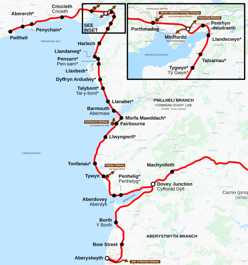
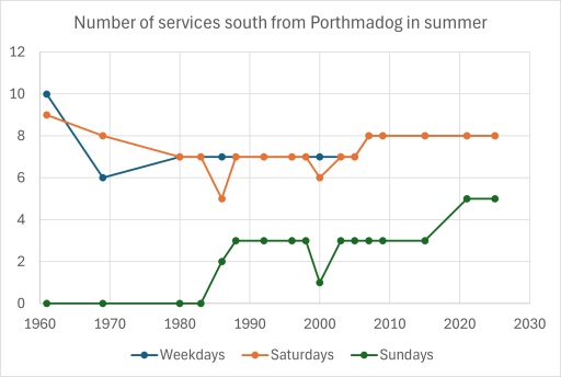
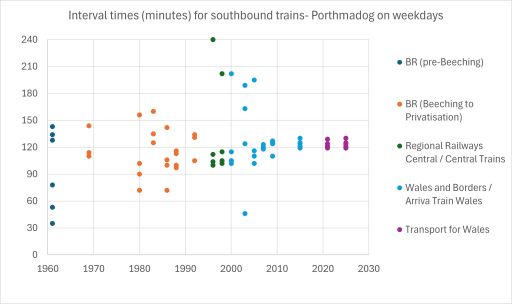
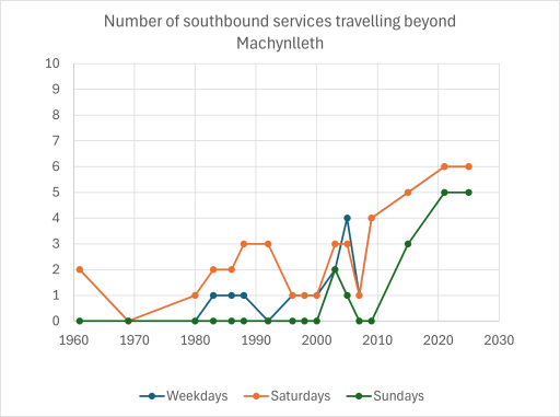
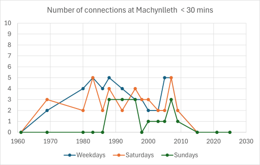
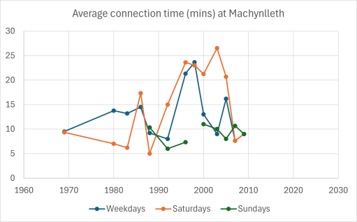
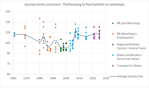
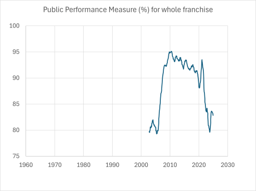
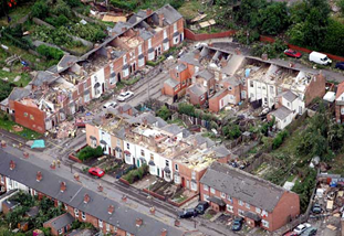
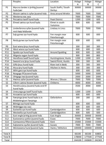
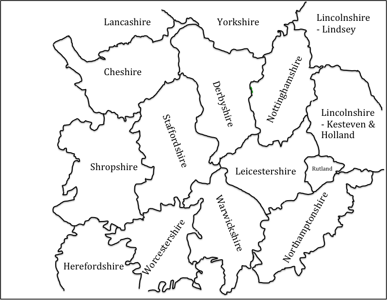
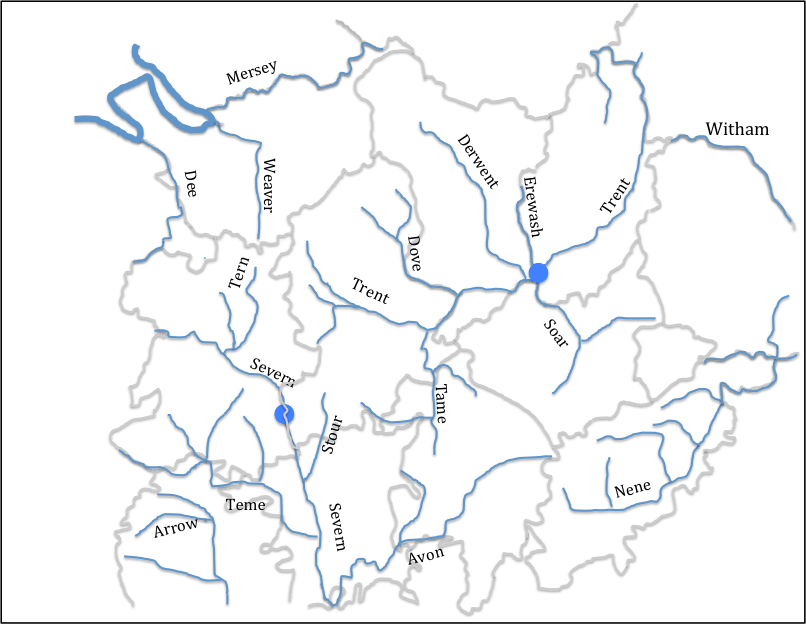
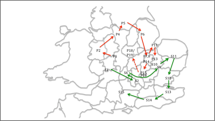
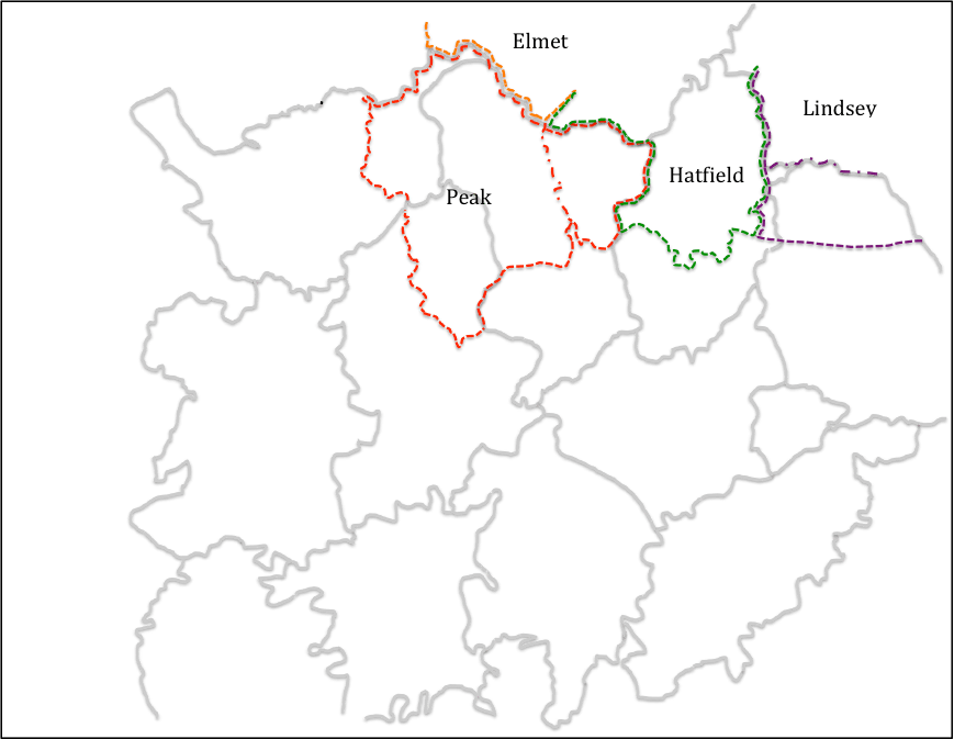
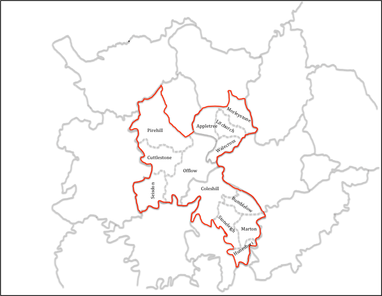
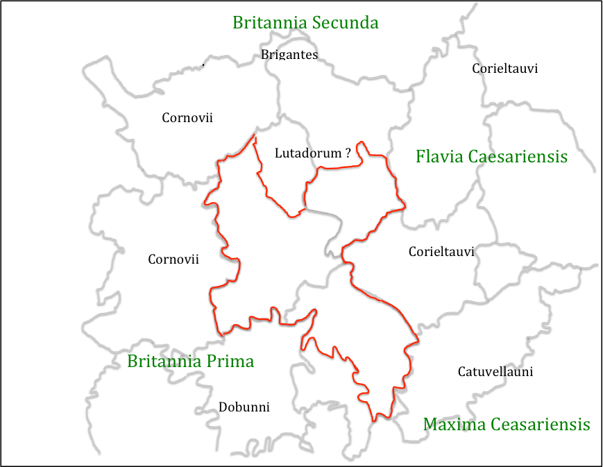
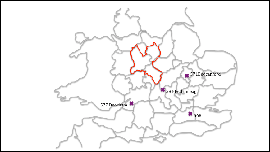
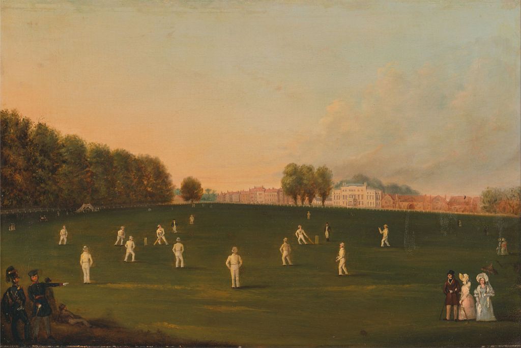
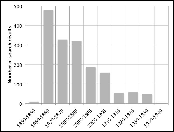
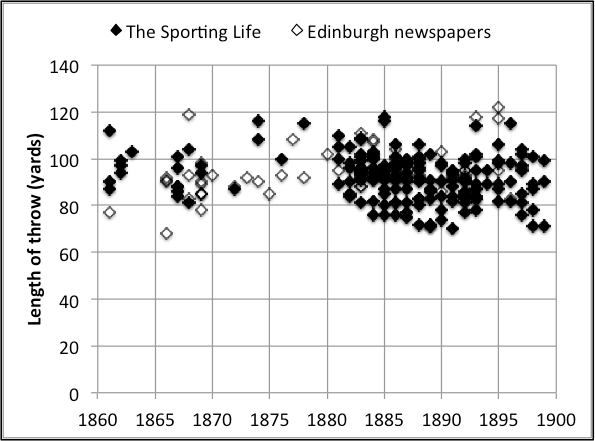
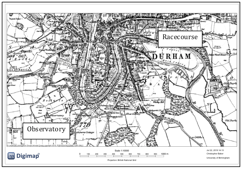
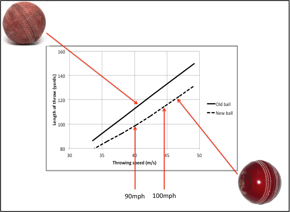
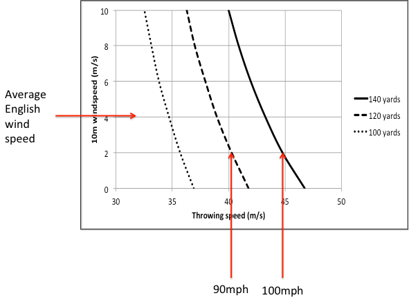
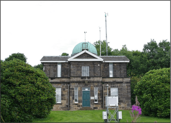
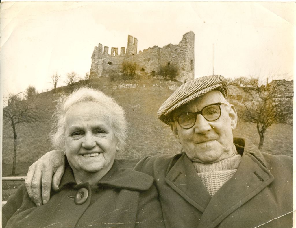
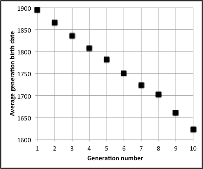
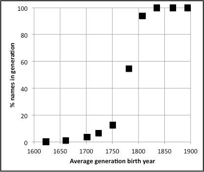
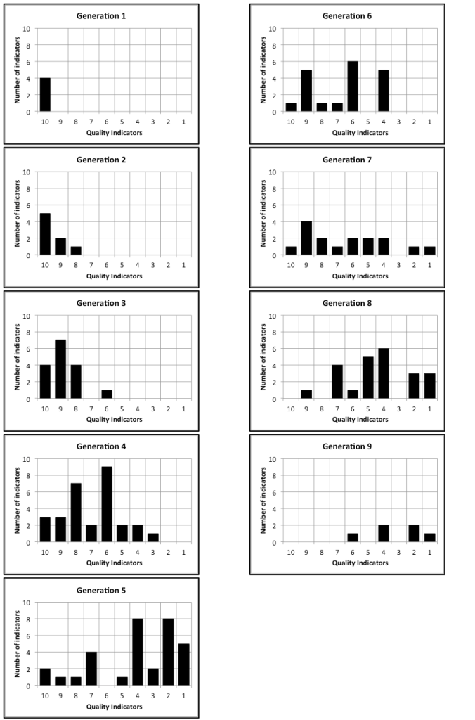