
When considering the effect of crosswinds on a new train, an obvious first step is to obtain data on the aerodynamic force and moment coefficients, usually through the use of wind tunnel tests, with the forces and moment coefficients being measured for a range of yaw (wind) angles from 0 to 90 degrees. This process however is not quite as straightforward as it sounds. The conventional approach is to use static models in a low turbulence wind tunnel. This approach of course models neither the relative motion between the train and the ground, nor the effects of atmospheric turbulence. It does however have the merits of simplicity and convenience. The conventional argument often used to justify this approach is that for high-speed trains, the relative motion between the train and the wind leads to the train experiencing low levels of turbulence. Whilst this is the case to some extent, it is not a wholly adequate argument. Figure 1, from Train Aerodynamics – Fundamentals and Applications (TAFA), shows how the turbulence length scale, turbulence intensity and velocity shear relative to the train vary with train speed for a 90 degree cross wind. Values are given as ratios of the values when the train is stationary. It can be seen that even at 400 km/h, the train still experiences a turbulence intensity of around 30% of its stationary value, which one might expect to have a not insignificant effect on the flow around the train,.
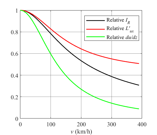
Figure 1 Variation of relative values of turbulence intensity (black), turbulence length scale (red) and shear (green) with train speed for a 90 degree cross wind (from TAFA)
An alternative approach would be to use a wind tunnel simulation of the atmospheric boundary layer in which to measure the train forces and moments. This of course is only really applicable to stationary trains. On the basis of figure 1, I argued in TAFA that low turbulence wind tunnel tests would be best for train speeds greater than 200 km/h and atmospheric boundary layer tests would be best for train speeds below that value – but that of course represents rather a messy compromise. And both methods fail to address the issue of train / ground relative motion.
So what are the alternatives? The first might be thought to be the use of CFD to properly model both atmospheric effects and train / ground motion. However, the simulation of a realistic scenario requires complex CFD methodologies (usually DDES) with very complex domain boundaries that include the specification of atmospheric turbulence. The calculation of the flow field for just one yaw angle takes several weeks on supercomputer systems, and in reality CFD calculations of this type tend to mirror the low turbulence wind tunnel tests.
In physical model terms, two alternatives present themselves. The first is the measurement of cross wind forces and moments on a moving model rig such as the TRAIN Rig owned by the University of Birmingham. Again, the experimental issues are formidable. The use of force balances within moving model rigs is not straightforward, and measurements of this type are usually made through the measurement of surface pressures with internal transducers, which because of transducer size and the need to carry out multiple runs to obtains stable average pressures requires multiple runs, with different pressure positions at any one yaw angle – a very tedious and complex process. An alternative would be to carry out conventional wind tunnel tests, but with a range of different turbulence simulations, each simulation being valid for one train speed only. The thought of such tests is enough to make wind tunnel operators consign it to the rubbish bin without much hesitation.
But the issue is important. Figure 2 shows three different sets of lee rail rolling moment coefficients for the Mark 3 coach, the GB benchmark vehicle that has run on exposed lines for many decades without incident. The three sets of coefficients are obtained from low turbulence wind tunnel tests; tests with an atmospheric boundary layer simulation with the coefficients formed from the mean values of measured forces and velocities; and those obtained from similar tests but with the coefficients formed from one-second peak values of forces and velocities (from Measurements of the cross wind forces on trains). The atmospheric boundary layer results are shown together with corresponding full scale results from field measurements on a real train. There can be seen to be significant differences between the three curves, particularly in the low yaw angle range which is important at high train speeds, with the low turbulence values being significantly above the atmospheric boundary layer values and the peak values being below the mean ones. If these coefficients are used to obtain cross wind characteristics (CWCs), which are plots of accident windspeed against vehicle speed, as outlined in another post and in TAFA chapter 11 and in a recent blog post, then the differences in acceptable windspeeds can be seen to be significant, particularly in the speed range around 200 km/h – see figure 3. Note that this plot shows train speeds of up to 400 km/h, which is wholly unrealistic for the Mark 3 coach – and certainly I wouldn’t care to be in one travelling at that speed! – but serves to illustrate the lack of agreement between the CWCs calculated using different moment coefficients. The difference in CWCs can be expected to make a significant difference to the calculation of accident risk, or to any operational restrictions that might be imposed, with the low turbulence results giving higher risk values and more severe restrictions.

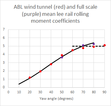
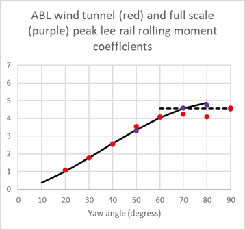
Figure 2. Lee rail rolling moment coefficients for Mark 3 coach
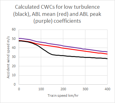
Figure 3 Crosswind characteristics for Mark 3 coach
I have to admit this is a problem that I have been mulling over on and off for many years (which gives a rather sad picture of the life I lead I fear). My thoughts have been basically around the idea of how to obtain representative force coefficients to allow for the major effect of atmospheric turbulence at low train speeds and the much smaller effect at high speeds, perhaps by some interpolation of the low and high turbulence coefficients. This is not simple however, as there is no direct correspondence between variation of these coefficients with yaw angle and variation with train speed.
But there is perhaps another way – and that is to consider not the force and moment coefficients, but rather the CWCs shown in figure 3. It seems reasonable to me to assume that the most representative CWC would lie somewhere between the low and high turbulence characteristics, lying close to the ABL curve at low train speeds, and close to the low turbulence curves at high train speed. Thus figure 4 shows the CWCs formed from giving a variable weighting to the low and high turbulence curves at different train speeds, with a 100% weighting given to the low turbulence curves at a train speed of 0 km/h, and a 0% weighting at a train speed of 400 km/h, with a linear variation in between. More sophisticated weighting variations could be considered, but this approach is adequate for illustrative purposes. The two curves of figure 4 are for the interpolation of the CWCs calculated from the mean and peak coefficients with those obtained from the low turbulence coefficients. It can be seen that this approach significantly raises the CWCs in the mid speed range from the low speed values and will thus result in substantial risk reduction.
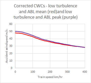
Figure 4. Interpolated cross wind characteristics
Up to now, I have referred to potential risk reductions in rather broad terms. It is however possible to put some numbers to these statements. Table 1 shows the accident wind speed at a train speed of 200 km/h for each of the above CWCs and the associated risk at the reference site as defined in my earlier post. For the original CWCs derived from the ABL coefficients, , the risks is of the order of 10-7 to 10-8, but for the CWC derived from the low turbulence conditions, the risk approaches 10-5 – almost two orders of magnitude greater. Whilst the absolute values of risk are quite arbitrary, it is clear that the use of the low turbulence characteristic would lead to a much more pessimistic (and perhaps unrealistic) risk assessment, and lower than necessary wind speed restrictions. The interpolated CWCs give values of risk of ca little less than 10-6, roughly midway between the atmospheric boundary layer and low turbulence values.

Table 1. Accident windspeeds and risk values for Mark 3 coach at a train speed of 200 km/h
So to conclude, the method outlined above gives a potentially realistic way of solving the problem of what type of wind tunnel test to use for train cross wind risk assessment. It requires two sets of wind tunnel experiments, one with low turbulence and one with an atmospheric boundary layer simulation, which is a more complex methodology than at present, but does not require extremely complex wind tunnel or CFD trials. The method results in lower values of calculated risk than would be the case using conventionally derived CWCs, and higher values of accident wind speeds.
