Tornadoes and debris

Get the facts about tornadoes - Chronicle Media

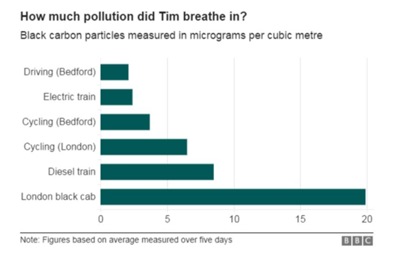
The debris trajectory animations of Figures 6 to 11 were provided by Professor Mark Sterling, whose ability to use advanced EXCEL functions seems to be significantly greater than mine. His contribution is much appreciated.

Previous work

In 2017 Mark Sterling and I published the paper “Modelling wind field and debris flight in tornadoes”, which described the integration of a tornado wind field model and the debris flight equations to look at the pattern of compact debris movement in tornadoes of different types. Typical results for falling and flying debris are shown in figure 1 below and give an indication of the complexity of the debris trajectories that were predicted.

Figure 1. Debris Trajectories from 2017 model

Now whilst the tornado wind model that was used in the analysis was a considerable improvement over those that existed at the time, in that it gave a consistent three dimensional velocity formulation, it did however have one major drawback. This was the fact that the vertical velocity component was unbound and increased with height, albeit quite slowly. In a more recent paper in 2020 “The lodging of crops by tornadoes”, we developed an improved model, in which the vertical velocity peaked at a certain height and then decreased at greater heights. In this blog post I will briefly explore  the use of this wind model to predict compact debris flight paths using the same methodology as in the first paper, and in doing so will illustrate the importance of the tornado model on debris trajectory prediction.

The tornado wind model

Figure 2. Velocities from 2020 model

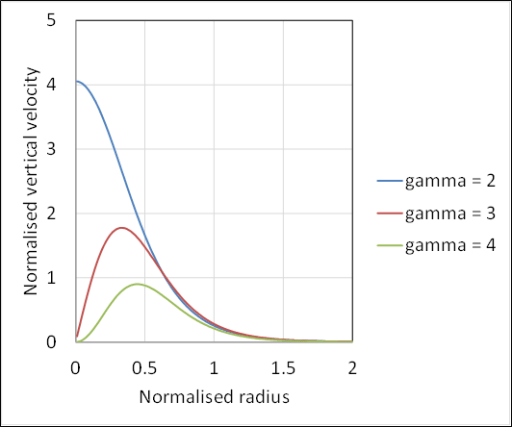
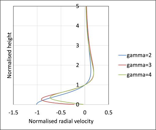
The expressions for the radial, circumferential and vertical velocities in the 2020 model are given in figure 2. Here the velocities are normalized by the maximum circumferential velocity and the radial and vertical distances by the radius at which the maximum velocity occurs. Note that this is different from the 2017 paper where the maximum radial velocity was used for normalization. The parameter K is related to what will be termed the swirl ratio S (the ratio of the maximum circumferential to maximum radial velocity) by a function of the parameter gamma, which is a shape parameter that affects the shape of the radial and vertical profiles. (Unfortunately this web template doesn’t support Greek letters, so I have to spell them out). Figure 3 shows typical velocity profiles for different values of this parameter.  It can be seen that for gamma = 2, the peak of the vertical velocity is at the vortex centre, as in a typical single cell vortex, whilst for higher values it moves away from the centre becoming more like a two cell vortex (but note there is no downflow at the vortex centre in this case.

Debris flight equations

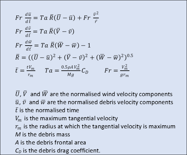
The equations for compact debris flight are given in figure 4. These are the same as in the 2017 paper, although expressed a little differently. The debris velocities (lowercase) in the three directions are again normalized by the maximum tangential tornado velocity. Two dimensionless parameter are identified – the Tachikawa number Ta that relates the flow force on the debris particle to its weight, and a tornado Froude number Fr. Different dimensionless parameters were used in the 2017 paper, because of the different reference velocity that was used

Figure 4. Debris flight equations

Solutions

Figure 5. Base case parameters

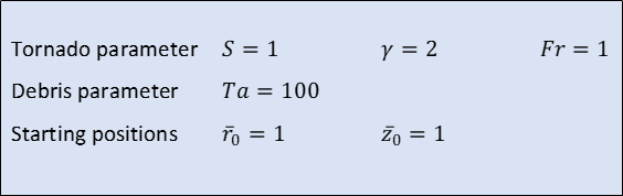
Putting together the velocity equations in figure 2 and the particle flight equations in figure 4, it can be seen that there are four parameter that define debris trajectories – the tornado parameters S, gamma and Fr, and the debris Tachikawa number Ta. In addition any one flight trajectory will be defined, at least in its early stages by the dimensionless values of the radius and height at its release point. If these six parameters are specified then the equations of debris flight can be solved in a straightforward manner.  In what follows we define a base case situation as in figure 5, and then vary each of the parameters around this base case value. We present the results in the animations of figures 6 to 11.Each animation shows four plots – the trajectories projected onto a vertical plane through the tornado centre; the trajectories projected onto a horizontal plane; the trajectories in a rotating plane in the radial and vertical directions, and a plot of the variation of particle kinetic energy with time. The latter acts as a damage indicator of debris flight, but also clearly shows whether or not the solution converges or diverges with time. Note that the dimensionless time shown in the kinetic energy plots is proportional to the time of revolution of the vortex – a time of 2 pi corresponds to one vortex revolution. 

aaaaaaaaaaaaaaaaaaaaaaaaaaaaaaaaaaaaaaaaaaaaaaaaaaaaaaaaaaaaaaaaaaaaaaaaaaaaaaaaaaaaaaaaaaaaaaaaaaaaaaaaaaaaaaaaaaaaaaaaaaaaaaaaaaaaaaaaaaaaaaaaaaaaaaaaaaaaaaaaaaaaaaaaaaaaaaaaaaaaaaaaaaaaaaaaaaaaaaaaaaaaaaaaaaaaaaaaaaaaaaaaaaaaaaaaaaaaaaaaaaaaaaaaaaaaaaaaaaaaaaaaaaaaaaaaaaaaaaaaaaaaaaaaaaaaaaaaaaaaaaaaaaaaaaaaaaaaaaaaaaaaaaaaaaaaaaaaaaaaaaaaaaaaaaaaaaaaaaaaaaaaaaaaaaaaaaaaaaa

Figure 6. Effect of variations in Tachikawa number

First consider the effect of changing Tachikawa number, Ta – see Figure 6. This represents changes in the nature of the debris. A low value of Ta represents heavy debris and vice versa. It can be seen that at low values of Ta, the debris tracks can reach significant heights and the debris undergoes a diverging motion when viewed in the radius / height plane, with a diverging kinetic energy oscillation. At some point in the trajectory the debris hits the ground and the energy falls to zero. The base case situation at Ta = 100 is still mildly diverging but the trajectory does not intersect the ground plane for the length of the calculation. As Ta increases further, the debris takes up a stable path in the radius / height plane travels around a small circular trajectory, with the kinetic energy converging to a stable value. This suggest that light debris can reach an equilibrium where it is held aloft by the tornado. The position around which the circular motion takes place is around a normalized radius of 1.3 and a normalized height of 0.9. The value of height is much less than calculated in the 2017 paper, reflecting the fact that the vertical velocity does not decrease indefinitely with height for the new model as it did in the old.

aaaaaaaaaaaaaaaaaaaaaaaaaaaaaaaaaaaaaaaaaaaaaaaaaaaaaaaaaaaaaaaaaaaaaaaaaaaaaaaaaaaaaaaaaaaaaaaaaaaaaaaaaaaaaaaaaaaaaaaaaaaaaaaaaaaaaaaaaaaaaaaaaaaaaaaaaaaaaaaaaaaaaaaaaaaaaaaaaaaaaaaaaaaaaaaaaaaaaaaaaaaaaaaaaaaaaaaaaaaaaaaaaaaaaaaaaaaaaaaaaaaaaaaaaaaaaaaaaaaaaaaaaaaaaaaaaaaaaaaaaaaaaaaaaaaaaaaaaaaaaaaaaaaaaaaaaaaaaaaaaaaaaaaaaaaaaaaaaaaaaaaaaaaaaaaaaaaaaaaaaaaaaaaaaaaaaaaaaaa

Figure 7. Effect of variations in Froude number

The effect of variations in Froude number is shown in Figure 7. The primary effect that increase in Fr has is to increase the centrifugal force on the debris. At low values, the trajectories are stable and similar to that of the base case. As the values increase above 1.0 the oscillations become larger due to the increased centrifugal forces and eventually become unstable, with the trajectories meeting the ground at high values.

aaaaaaaaaaaaaaaaaaaaaaaaaaaaaaaaaaaaaaaaaaaaaaaaaaaaaaaaaaaaaaaaaaaaaaaaaaaaaaaaaaaaaaaaaaaaaaaaaaaaaaaaaaaaaaaaaaaaaaaaaaaaaaaaaaaaaaaaaaaaaaaaaaaaaaaaaaaaaaaaaaaaaaaaaaaaaaaaaaaaaaaaaaaaaaaaaaaaaaaaaaaaaaaaaaaaaaaaaaaaaaaaaaaaaaaaaaaaaaaaaaaaaaaaaaaaaaaaaaaaaaaaaaaaaaaaaaaaaaaaaaaaaaaaaaaaaaaaaaaaaaaaaaaaaaaaaaaaaaaaaaaaaaaaaaaaaaaaaaaaaaaaaaaaaaaaaaaaaaaaaaaaaaaaaa

Figure 8. Effect of variation in Swirl Ratio

The effects of variations in the Swirl ratio shown in Figure 8 are complex, with diverging trajectories (and ground impact) at both low and high values, and a region of stable trajectories between values of around 1.0 to 1.9. At low values the trajectories are destabilized by the high values of radial velocity, and at high values are destabilized by high values of the circumferential velocity.

aaaaaaaaaaaaaaaaaaaaaaaaaaaaaaaaaaaaaaaaaaaaaaaaaaaaaaaaaaaaaaaaaaaaaaaaaaaaaaaaaaaaaaaaaaaaaaaaaaaaaaaaaaaaaaaaaaaaaaaaaaaaaaaaaaaaaaaaaaaaaaaaaaaaaaaaaaaaaaaaaaaaaaaaaaaaaaaaaaaaaaaaaaaaaaaaaaaaaaaaaaaaaaaaaaaaaaaaaaaaaaaaaaaaaaaaaaaaaaaaaaaaaaaaaaaaaaaaaaaaaaaaaaaaaaaaaaaaaaaaaaaaaaaaaaaaaaaaaaaaaaaaaaaaaaaaaaaaaaaaaaaaaaaaaaaaaaaaaaaaaaaaaaaaaaaaaaaaaaaaaaaaaaaaaa

Figure 9 Effect of variations in gamma

The change in values of gamma from the one cell form of gamma = 2 to the quasi-two cell form of gamma = 4 shown in Figure 9 results in little change to the debris trajectories from the base case, although the oscillations in the kinetic energy fall as gamma increases.

aaaaaaaaaaaaaaaaaaaaaaaaaaaaaaaaaaaaaaaaaaaaaaaaaaaaaaaaaaaaaaaaaaaaaaaaaaaaaaaaaaaaaaaaaaaaaaaaaaaaaaaaaaaaaaaaaaaaaaaaaaaaaaaaaaaaaaaaaaaaaaaaaaaaaaaaaaaaaaaaaaaaaaaaaaaaaaaaaaaaaaaaaaaaaaaaaaaaaaaaaaaaaaaaaaaaaaaaaaaaaaaaaaaaaaaaaaaaaaaaaaaaaaaaaaaaaaaaaaaaaaaaaaaaaaaaaaaaaaaaaaaaaaaaaaaaaaaaaaaaaaaaaaaaaaaaaaaaaaaaaaaaaaaaaaaaaaaaaaaaaaaaaaaaaaaaaaaaaaaaaaaaaaaaaa

Figure 10. Effect of variations in radial starting position

aaaaaaaaaaaaaaaaaaaaaaaaaaaaaaaaaaaaaaaaaaaaaaaaaaaaaaaaaaaaaaaaaaaaaaaaaaaaaaaaaaaaaaaaaaaaaaaaaaaaaaaaaaaaaaaaaaaaaaaaaaaaaaaaaaaaaaaaaaaaaaaaaaaaaaaaaaaaaaaaaaaaaaaaaaaaaaaaaaaaaaaaaaaaaaaaaaaaaaaaaaaaaaaaaaaaaaaaaaaaaaaaaaaaaaaaaaaaaaaaaaaaaaaaaaaaaaaaaaaaaaaaaaaaaaaaaaaaaaaaaaaaaaaaaaaaaaaaaaaaaaaaaaaaaaaaaaaaaaaaaaaaaaaaaaaaaaaaaaaaaaaaaaaaaaaaaaaaaaaaaaaaaaaaaa

Figure 11. Effect of variations in vertical starting position

The debris trajectories remain stable as the normalized radius varies between 1 and 1.9 but outside those limits the trajectories diverge and intersect with the ground (Figure 10). Similarly the trajectories are only stable for normalized values for height between 0.8 and 1.2 (Figure 11). Thus the starting point window for the trajectories to ultimately attain a stable form is quite small.

Concluding remarks

A number of points arise from the results presented above.

  • Even for the simple wind and debris flight formulation adopted, debris trajectories can be quite complex.
  • A comparison of the results obtained with the old and the new wind field model show very considerable differences, due to the different vertical velocity formulation. analysis reveals that the debris trajectories can be specified by a small number of debris and tornado parameters, with the Tachikawa number and the Swirl Ratio being the most significant.
  • There are regions within parameter space for which the debris trajectories become stable – i.e. the debris flies indefinitely.

Pollution, Covid and Trains

Voyager at Birmingham New Street

There has been a significant amount of research recently to investigate the air quality in railway stations. Perhaps the major study, with which I was very much involved, involved extensive measurements of the air quality at Birmingham New Street by colleagues at the University of Birmingham (Figure 1). Measurements were made of the oxides of nitrogen (NOX) and particulate matter (PM) and concentrations were measured that were considerably in excess of Environmental Health limits. Typical daily average results are shown in Figure 2. This work informed the efforts by Network Rail to improve the air quality at the station through an improved ventilation system. Further work was carried out by Kings College London and Edinburgh University, under an RSSB contract, to measure NOX and PM at Kings Cross in London and Edinburgh Waverley. Typical results are shown in figure 3 and although these results are not as extreme as the Birmingham measurements, do show some exceedances of environmental health limits. Between them, these three investigations have given a great deal of information on station air quality and informed methods for alleviating the worst of the effects.

Figure 1. Air quality measurements at Birmingham New Street
Figure 2. Daily pollutant levels at Birmingham New Street (red lines show EU limits)
Figure 3 Comparison of pollutant levels at New Street, Kings Cross and Edinburgh Waverley

However, that is not the whole story. There are growing indications that air quality ON trains is also very poor. A study on diesel commuter stock in Canada has shown high levels of ultrafine particles and black carbon within the passenger cabins (Figure 4). In 2016 the BBC reported the measurements made by their reporter Tim Johns  as he commuted into London, which again showed high particulate levels on diesel commuter trains, although not as high as in Black Cabs (Figure 5). Similarly, the BBC in 2019 reported a study by the Committee on the Medical Effects of Air Pollutants which showed very high levels of particulates on the London underground (Figure 6) which resulted in a strong response from the rail unions. These high levels are presumably due to two sources – diesel particulate emissions from trains being ingested into air conditioning systems, and also from ambient particulates in the dirty tunnels of the underground. The levels of particulates measured have significant implications for human health, particularly for those with respiratory conditions.  

Figure 4. Air Quality measurements on Canadian trains
Figure 5. Particulate measurements by BBC Reporter
Figure 6. BBC report on Underground particulate levels

Similarly, some work has been recently reported from Greece that shows elevated levels of both gaseous pollutants and particulate pollutants on diesel trains, both in excess of EU limits (Figure 7). Again this is presumably due to ingestion of diesel emissions by ventilation systems. Hopefully in the near future we will see the results of more quantitative investigations for the UK of on train NOX and particulate concentrations, and of work to investigate the ingestion of external pollutants, both from diesel emissions and dirty environments, by ventilation systems. However current indications are, that, care should be taken in using ventilations systems that draw external air into the train without the use of extensive filtering of the input.

Figure 7. NOX measurements on Greek train (red line is EU limit)

And then along comes Covid-19. The importance of high levels of ventilation on reducing pathogen concentrations and thus the risk of infection is becoming clear – se for example the recent seminar organized by the University of Birmingham. Ideally, very high (airline) levels of air exchange with the outside are required in internal environments, including trains and buses. An interesting illustration of this is provided by the publicity material in figure 8 produced by SNCF in France. I have seen nothing similar for the UK. There is an obvious dichotomy here between the need to reduce external air intake to minimize NOX and PPM ingestion and to keep internal levels of NOX and particulates at an acceptable level, and the need to increase ventilation rates to decrease pathogen levels. Both could be achieved by aggressive filtration of the air drawn through the train. However, this is likely to require major modification to existing trains in Britain, that won’t be cheap. I suspect train ventilation is going to become a major issue in the near future.

Figure 8. SNCF publicity material

Modelling of extreme wind gusts

Nomenclature

This post addresses the issue of the use of what has become known as the “Chinese Hat” gust model. The use of this title has become increasingly problematic over recent years for obvious reasons, and I will no longer use it, but will instead refer to the “CEN extreme gust model” in what follows.

The CEN extreme gust model

In a number of situations in wind engineering, some sort of deterministic (as opposed to stochastic) gust model is required in order to determine structural response. One such case is in the determination of the risk of overturning of road or rail vehicles in high winds. A methodology of this type is set out in CEN (2018), where an extreme gust model is described.  This model was originally developed in wind loading studies for wind turbines as a time dependent gust to be applied to calculate wind turbine loading at one fixed location (Bierbooms and Cheng, 2002). As such, it is perfectly adequate and a good representation of an average extreme gust in high wind conditions.  In the methodology of CEN however, it is re-interpreted as a stationary spatially varying gust. This must be regarded as a very significant assumption for which, in my view, there is little justification. Nonetheless the formulation has proved useful practically and we begin by considering it in a little more detail.

For a wind normal to the track, the extreme gust formulation is given by equation (1) on Box 1. Note that the “characteristic frequency” of the gust is calculated from standard wind engineering methods for temporally, rather than spatially, varying gusts. Equation (1) is a generalised form of that given in CEN (2018) to remove some of the constants that tie the expression to a particular location and topography through specific values of peak factor and the turbulence intensity (the ratio of the standard deviation to the mean velocity). The time dependence is recovered through the passage of the train passing through this gust at a speed v = xt to give equation (2). It can be seen that the gust thus has a maximum value of (1+ peak factor x turbulence intensity) when t = 0 and decreases to unity for small and large times. It is symmetrical about t = 0. The velocity relative to the train is then found by the vector addition of this gust velocity with the vehicle velocity to give a time varying value.

To enable the gust profile to be specified, the characteristic frequency f is required. This is specified in equations (3) to (5). These equations are again in a more generalized form than given in CEN (2018), where a value of the upper limit of integration is fixed at 1 Hz, together with an implicit value of the turbulence length scale of around 75m. The genesis of the 4.18 factor is however not clear to me.  Equation (3) shows that the calculation of the characteristic frequency is thus based on the calculation of the zero-crossing rate of temporal fluctuations through the use of the velocity spectrum. Again, note that these parameters describe a time varying rather than a spatially varying velocity, and their use is not formally consistent with a spatially varying gust. From equations (3) to (5), it can be seen that the normalized characteristic frequency is a function of the normalized upper limit of integration. A numerical solution of these equations was carried out and the following empirical line fitted to the results for a value of the latter greater than 1.5 (which is the realistic range) – equation (6). From equations (2) and (6) we thus obtain equation (7). Although the overall methodology cannot be regarded as wholly sound, equation (7) does (in principal) significantly simplify its use and also allows the implicit wind parameters in the method to be explicitly defined.

Box 1 Equations 1 to 7

Is there a better methodology?

It can be seen from the above that the CEN  methodology thus does not fully describe a typical gust as seen by a moving train, which would vary both spatially and temporally, and can at best be regarded as an approximation, although its practical utility must be acknowledged. Ideally, if such an approach is to be used, a gust that varies both in space and time is really required.  Such a gust was used in the SNCF route assessment method of Cleon and Jourdain (2001), where the shape of the gust is appropriately described as a rugby ball. This method was however for very specific wind characteristics and does not seem to have found widespread use. Thus in this post, we investigate the possibility of developing a spatially and temporally varying gust, that can be expressed in a simple form (ideally similar to equation (2)) for practical use.

Towards a new model

In this section we will draw on experimental results for extreme gust characteristics in both temporal and spatial terms to construct a simple, if empirical model, that fulfills the function of the CEN (2018) model without the theoretical drawbacks.

We consider first the full-scale experimental data analysed by Sterling et al (2006) which used conditional sampling to determine the average 99.5th percentile gust profile for four anemometers on a vertical mast with heights between 1m and 10m. These results thus give the time variation in gust speed as the gust passes the anemometers. They showed that the gust profiles could be well approximated by the formula shown in equation (8) (Box 2). The parameter G in this equation is the equivalent of the peak factor multiplied by the turbulence intensity in equation (2) and for these measurements was 0.786.  n was -0.096, and the value of m depended upon whether t was greater or less than zero. For t < 0, i.e. on the rising limb, m was 0.1, whilst for t > 0, on the falling limb, m was 0.2. The gust shape was thus asymmetric with a maximum at t = 0.  This curve was a good fit to all the gust profiles throughout the height range. In what follows we will use a rather different curve fit expression to the same data, more consistent with that used in CEN (2018) – equation (9). It was found that the best fit value of b  was equal to 0.5 for all t, whilst the best fit values of a were 0.49 for the rising gust and 0.37 for the falling gust. This expression thus describes the temporal variation of wind speed as a gust passes through the measuring point

To describe the lateral spatial variation of the gust profile, we use the data of Baker (2001) who presents conditionally sampled peak events for pressure coefficients along a 2m high horizontal wall. This data allows the lateral extent of the gusts to be determined, from the variation of the time varying pressure coefficient divided by the mean value of the coefficient and then assuming that the gust velocity variation can be found from equation (10). The spatial variations of velocity were then fitted by a curve of the form of equation (11). g was found to be 6.16 and d was found to be 0.7.

On the basis of the above expressions one can thus write the expression of equation (12), which describes the variation of the gust velocity in both space and time. The movement of the train through the gust can again be allowed for by letting x = vt (equation (13)).

Box 2 Equations 8 to 13

Model comparison

Box 3 sets out the formulations of the CEN extreme gust model and the model derived here. In some ways they are similar in form, with an exponential formula that is primarily a function of normalized time. Whilst the CEN model is symmetric around t = 0, the new model has a degree of asymmetry because of the different values of the curve fit parameters for t < 0 and t > 0. However an examination of the new model suggest that the asymmetric term may be small, and thus Box 3 also shows an approximate version of the new model where this term is neglected.

Box 3 Model Summary

Figure 1 shows a comparison of these three models for the following parameter values – peak factor = 3.0; turbulence intensity = 0.25; train speed = 75m/s; mean wind speed = 25m/s; turbulence length scale = 75m, upper frequency of integration = 1.0Hz. It can be all three models are similar in form, showing a sharp peak at t = 0. The full and approximate forms of the new model are almost indistinguishable, showing that the approximation suggested above is valid. The main difference is that the CEN model has a much greater spread in time than the new model. This difference persists whatever input parameters are chosen.

Figure 1 Model Comparison

At this point it is necessary to consider again the genesis of the models – the CEN model resulted from an application of a time varying gust model as a spatially varying gust model, whilst the new model was developed based on measured temporal and spatial gust values. As such, I would expect the latter to be more accurate. The broad spread of the CEN gust may result from an application of the time varying along wind statistics to a cross wind spatial gust. Since it is known that that longitudinal integral scale is several times larger than the lateral integral scale, this would result in a wider spread of the gust than would be realistic. This is to some extent confirmed by the period of the two gusts – around 2s for the CEN gust and around 0.8s for the new model. For a train speed of 75m/s, this corresponds to gust widths of 150m and 60m – roughly approximating to the expected the longitudinal and lateral turbulence integral scales.

Concluding remarks

In this post I have looked again at the CEN extreme gust method and raised concerns about its fundamental assumptions. I have also developed an equivalent, but perhaps more rigorous, methodology based on experimental data for wind conditions at ground level. This strongly suggests that the CEN gusts are spatially larger than they should be, which suggests its long term use should be reviewed. However, when used to compare the crosswind behaviour of individual trains, rather than in an absolute sense, it is probably quite adequate.  

References

Baker C J, 2001, Unsteady wind loading on a wall, Wind and Structures 4, 5, 413-440. http://dx.doi.org/10.12989/was.2001.4.5.413

Bierbooms, W., Cheng, P.-W., 2002. Stochastic gust model for design calculations of wind turbines. Journal of Wind Engineering and Industrial Aerodynamics 90 (11), 1237e1251. https://doi.org/10.1016/S0167-6105(02)00255-6.

CEN, 2018. Railway Applications d Aerodynamics d Part 6: Requirements and Test Procedures for Cross Wind Assessment. EN 14067-6:2018.

Cleon, L., Jourdain, A., 2001. Protection of line LN5 against cross winds. In: World Congress on Rail Research, Köln, Germany.

Sterling M, Baker C, Quinn A, Hoxey R, Richards P, 2006, An investigation of the wind statistics and extreme gust events at a rural site, Wind and Structures 9, 3, 193-216, http://dx.doi.org/10.12989/was.2006.9.3.193

Some musings on tornado vortex models

From Wikipedia

Recently I have been considering the fundamental nature of a range of analytical models of tornado like vortices, and have written up my musings as an extended essay that can be read and downloaded below. In the essay I look at the class of tornado models that are solutions of the Navier-Stokes or Euler equations. It is clear that they all share a common analytical basis based on the assumption, either implicit or explicit, that the three velocity components (radial, vertical and circumferential) can each be specified by the multiple of two functions – one a function of radius only, and one a function of height only. Assumptions are made concerning the nature of one particular velocity component, and this assumption then allows the other components to be calculated from the continuity and momentum equations via the method of separating the variables. The recognition of this commonality allows a common analytical formulation to be developed that underlies all the models.

Those models that are solutions of the full Navier-Stokes equations (the Burgers-Rott, Sullivan and Vasistas et al models) derive velocity component formulae that are functions of Reynolds number. In the context of a full-scale tornado, this is a Reynolds number based on turbulence eddy viscosity rather than molecular viscosity. The assumptions required to obtain analytical solutions result in vertical velocities that are unbound with height and in some cases radial velocities that are unbound with distance from the vortex centre.  

Those models that are solutions of the Euler equations (two by Baker and Sterling  and two new models A and B) have, on the whole, rather more realistic formulations of the velocity components and, with one exception, all components for these models are bound in the vertical and radial directions. Instead of the Reynolds number, the velocity components are functions of constants of integration that relate to the Swirl ratio – the ratio of the maximum circumferential to radial velocities. As the circumferential velocity profiles in these models fall to zero at ground level in a reasonably realistic way, the boundary layer at the bottom of the tornado is modeled to some extent. The common analytical framework of these models allows, in principle, the derivation of a large number of different models, provided that they are of a form that allows the solutions to be obtained through simple integrations.  However the drawback of such models is that the pressure is zero at the ground for all distances from the vortex core and thus the dip in pressure at the centre of tornadoes is not modeled. This is broadly a consequence of viscous effects not being properly modeled near the ground. 

Whilst most of the models represent single cell tornado vortices, two of them – those of Sullivan and new model B – give solutions for two cell vortices. The essay shows that the Sullivan model, based on the Navier-Stokes equations, has a more general form than that given in the original paper and can model one-cell and two-cell vortices and the transition between them. New model B, based on the Euler equations is also able to model both sorts of vortex.  

The essay concludes that further work is required in two areas. Firstly there is a need to develop methods that do not rely on the assumption that the velocity components are multiples of two functions – one of radius and one of height – as recent experimental data suggests that the vortex radius can vary significantly with height. Secondly, the tornado boundary layer needs to be modeled in a more satisfactory way than at present, and the essay suggest that this might be done through matching a viscous solution of the Navier-Stokes equation near the ground, with an inviscid solution from the Euler solution away from the ground.  I may have more to say on this in the future.

Measuring the behaviour of pedestrians in high winds

This post outlines some of the results from the project “The safety of pedestrians, cyclists and motor vehicles in highly turbulent urban wind flows” funded by the UK Engineering and Physical Sciences Research Council. The work that is described below involved a number of colleagues, whose contribution to the project was significantly greater than mine, particularly Dr Zhenru Shu, Dr Mike Jesson, Dr Andrew Quinn, and Prof Mark Sterling. Their contribution is gratefully acknowledged.

1. Introduction

The assessment of wind conditions around new buildings has become standard practice over recent years, either by wind tunnel testing or through the use of CFD calculations. The assessments usually concentrate on two aspects – the effect of wind conditions on human comfort and thus the usability of the area around the building; and the effect of high wind conditions on human safety and stability. It is with the latter that this paper is concerned. In general the criterion for assessing a site for pedestrian safety is based on a gust wind speed of a specified magnitude with a specified probability of occurring, that is deemed to be at the safety limit. Current UK practice is illustrated in Figure 1 below. There is a great deal of variability in the specification of this windspeed and the specification is usually based on largely subjective data from questionnaires etc. Following a fatality caused by high winds around a new building in the city of Leeds, a major research project was funded by the UK Engineering and Science Research Council to enable the University of Birmingham to investigate the safety of vehicles and pedestrians around high-rise buildings. This included full-scale wind measurements and the assessment of the ability of different wind tunnel and CFD techniques to replicate these measurements. In addition tests were carried out to make quantitative measurements of human response in gusty winds, using instrumentation mounted on volunteers. As will be appreciated by any reader who has tried to make full scale wind measurements of any type, the setting up of the experimental apparatus usually guarantees that strong winds will not occur, and the same phenomenon was observed for these tests. The two winter seasons that were available for these measurements had relatively few storms, and only two trials could be carried out. As a result, although some very interesting results were obtained and will be presented in what follows, they must be regarded as provisional and tentative. More work is required to obtain a fuller dataset of human response measurements of the type that are presented here.

Figure 1 Current UK practice for specifying wind comfort and safety (Values given are for mean wind speed and percentage of time exceeded)

2. The trials

Figure 2. The test site showing the walking route along the Biosciences building and the reference anemometer site on the Moorhead Tower

The trials on the response of pedestrians to high winds were carried out on the campus of the University of Birmingham (figure 2). A walking route of length 63m was set up in the centre of the campus. Eight sonic anemometers were placed 2m above the ground at 9m intervals along the route.  A reference anemometer was installed at the top of the nearby high rise Muirhead Tower. A reference anemometer was mounted at the top of the Moorhead Tower. All the anemometers sampled at 10 samples / sec, and data was recorded on an AntiLog data logger. Human response was measured using GaitUp Physilog (combined accelerometer and gyroscope) sensors. Sensors were attached to both feet of the subjects, and provided details of walking speed and stride parameters every second through GaitUp’s proprietary software. A third sensor was placed on the back of a safety jacket worn by the subjects and thus gave details of upper body acceleration.  

Two trials were carried out – October 2017 during Storm Ophelia, and in February 2019 (figure 3. In total there were 15 subjects, with weights ranging from 54 to 110kg, and ages between 28 and 75. Each subject was asked to walk along the test route 10 times in each direction during which the gait and acceleration information was measured. 

Figure 3 Wind conditions during the trials

3. Analysis

The overall wind conditions at the reference site on the Muirhead Tower are shown in figure 3 for the two test periods. It can be seen that in each case the wind is from the South-West (shown in longer term analysis to strongly be the prevailing wind direction), with gust speeds up to 18m/s

Before the data could be analysed, some data preparation was required. Firstly the gait data and accelerometer time series had to be synchronized with the anemometer time series of velocities and the raw accelerometer data was transformed into horizontal and vertical co-ordinates. The time series of velocity and direction relative to the subjects were then derived form the stationary anemometer data as the subject walked along the route. A histogram of gust speed distribution, as experienced by the volunteers, for the two trials is shown in figure 4.

Figure 4 Histogram of gust velocities

Initial inspection of the data showed that there was very significant variability between each recorded walk along the track. This was in part due to the normal variation in wind conditions with higher gust speeds on some walks than on other, but it also seemed that the reaction of subjects varied both with time and between subjects. A typical set of results is shown in figure 5.  The direction of travel of the subject is from 0 to 63m. The wind speed relative to the subject can be seen to have a maximum of around 12 m/s in this case (associated with the corner flow from an adjacent building). The horizontal and vertical accelerometer data show slight oscillations around the gust position gust with the former having an average value of zero, and the latter an average value of 1.0. Most of the gait measurements (cycle time, stride length, stride speed) revealed little change in behaviour as the subjects walked along the route, all remaining approximately constant along the walk in most conditions.  The one parameter that did show variation was the swing width – the lateral variation of the foot during a stride cycle. In particular rapid changes in swing width were sometimes (but not always) observed as the subjects encountered gusts – see the graph for swing width gradient.

Figure 5 Wind, acceleration and gait parameters for typical gust (green symbols indictate left foot, blue symbols indicate right foot)

At the highest gust speeds that were recorded, there were three events where the subject became unstable to a variable extent. Figure 6 shows the experimental data for one such case. Here it can be seen that at the gust position there are significant vertical and horizontal acceleration responses, and all the gait parameters show a response at the event. The swing width response is again the most noticeable.

Figure 6 Wind, acceleration and gait parameters for strong gust

A somewhat more quantitative approach to the data is possible by looking at the various responses statistically. In what follows we consider the results from both trials, for all subjects, as one dataset. Figure 7 shows the percentage of such gusts in which the subjects showed a swing width response (with either the left or right swing width changing by more than 0.06m in one second) and acceleration response (where an acceleration response greater than 0.05g could be detected) or an instability response (with an acceleration response greater than 0.4g). In considering these results the low number of gust events in the upper velocity bands need to be considered, as does the subjectivity of the response limits used. These points being made, it can be seen that for even low speed gusts of magnitude less than 10m/s, around 50% of the gusts result in a swing width response (which are mostly unconscious responses not registered by the subject). The frequency of such responses rise rapidly for gust speeds above 10 m/s, and all gusts over 14 m /s show such a response. Acceleration responses become significant at gust speeds of about 10m/s, and are observed for all gusts above 16m/s. Instability responses begin to occur at gust speeds over 14m/s, although it should be noted here that only a very small number of such events (3) were observed.

Figure 7 Frequency of different types of response

4. Concluding remarks

The results for human response in gusts presented here suggest that three levels of response can be identified – swing width response , upper body acceleration response and instability response, with the frequency of each such response increasing with wind speed. However it must be emphasised once more that the number of bot high speed gust events and the number of subjects was too small for a valid statistical analysis to be carried out, and more data is required before firmer conclusions can be drawn.

Vehicle restrictions during windy conditions on long span bridges

The Bridges

Around the UK, there area number of relatively long and high bridges across river estuaries, that all operate some sort of traffic restriction protocol in high wind conditions, to limit the risk of vehicle accidents. In this post, I will attempt to collate publically available information on these traffic restriction protocols to assess their similarities and differences.  It will be seen (surprisingly in my view) that this information is not at all easy to find and sometimes does not seem to be in the public domain. .

The bridges that will be considered are shown in Table 1, which gives name, location, construction type and length.  Pictures of them are given in figure 1. It can be seen that, with the exceptions of the Cleddau Bridge in South Wales and the Skye Bridge in Scotland, these are all over a kilometer long. The construction types vary, from concrete boxes on large numbers of concrete piers to long span suspension and cable stay structures. Only two bridges in the table have protection for vehicles against cross winds – the Prince of Wales (Second Severn) Bridge and the Queensferry Bridge in Edinburgh. All the bridges in the table have Wikipedia entries, which give further details of planning, construction and operation.

Table 1 The Bridges

Vehicle restrictions

The data for wind speed restrictions was found from a variety of sources – official documents, FOI releases, newspapers etc. The information that has been obtained is shown in Table 2. Most have a similar form, with different levels of restriction being used as the gust wind speed increases – vehicle speed limits, lane closures, restrictions to various classes of vehicles, and total closure. Most seem to base the wind speed values on local anemometers, although it is usually not clear where these are sited, and neither is the period of the gust given. Thus the values that are given are not strictly comparable with each other in absolute terms. 

Table 2 Wind speed restrictions 
(H- Headwind, C – Crosswind, * values are given in mph in table, but equivalent values in knots are used in practice)

From table 2 it can be seen that no data could be obtained for the Kessock Bridge, the Humber Bridge or the Prince of Wales (Second Severn) Bridge. With regard to the latter, vehicles crossing the bridge are shielded by wind fences and the bridge has not had to impose restrictions on traffic during its lifetime. Kessock probably has the same sort of traffic restriction strategy as the other Scottish bridges, as Transport Scotland operates a common approach. From press reports it seems that Humber has some sort of vehicle speed limit and high-sided vehicle restriction strategy, although it has not been possible to determine the wind speeds at which the different measures are put into place. . Also note that Queensferry has much higher values of wind speed for restrictions than the other bridges, again due to the fact that vehicles are protected by wind fences.

For the other bridges, there seems to be a general consistency in the information shown, with vehicle speed limits of either 30mph or 40mph imposed when the wind gusts over 35 to 50mph. Vehicle restrictions begin at gusts of around 45mph to 60mph, with double deck buses and high sided vehicles being restricted at the lower gust speeds. Further restrictions may be imposed on vehicles of different types, before overall bridge closure at wind speeds of 65 to 80mph. Some bridges use different gust speeds for cross winds and for headwinds. Orwell Bridge for example applies the crosswind criterion if the wind gust direction is from a sixty degree segment centred on the direction normal to the bridge. The Queen Elizabeth II Bridge at Dartford uses similar strategies to inform speed limits, lane closures, vehicle restrictions and bridge closure.

The restriction strategies depend very much on the nature of the traffic over the bridge and its location. For example, if only some vehicles are to be restricted, then some method of filtering them out and diverting them is required, which needs to take place at some distance from the bridge. Such procedures are in operation at Severn, Erskine, Humber and the Queen Elizabeth Bridges amongst others. Clearly ease of identification of vulnerable vehicles is required – see figure 2 for the Humber Bridge. Other bridges simply base their protocols on vehicle height eg 1.9m for Cleddau and 2.1m for Severn.

Description: Macintosh HD:Users:chrisbaker:Dropbox:Web site:Blog material:Crosswinds:Bridge closure:Humber.png
Figure 2 Humber Bridge High sided Definition

Orwell Bridge operates a very simple strategy, with different gust speed triggers for crosswinds and headwinds, leading to complete closure, without any restrictions for, say, high sided vehicles at lower wind speeds. This arises because of the urban nature of its surroundings, which makes vehicle filtering difficult. This has led to a considerable number of closures in recent years, and much public concern. Recently both numerical and wind tunnel studies have been carried out to investigate ways in which this strategy can be modified, perhaps through the use of speed limits, lane restrictions or barriers. The details of these studies have not been released to date but may prove of some interest. Studies to relax the restrictions on Skye Bridge have also been recently carried out following frequent closures and public complaints.

As can be seen, the various restriction strategies are in general quite simple and easy to operate. This inevitably means that they are conservative and largely based on the most vulnerable vehicle – usually unladen high sided vehicles. There are in fact methods available for discriminating between vehicle types and vehicle weights – see the recent paper by Baker and Soper (2019) for example. This gives a method for determining a curve of accident wind speed against vehicle speed for specific vehicle type and weight, based on which restrictions strategies for any particular vehicle can be determined. However operational constraints make the full utilisation of such methods difficult. Until such time as vehicle type and vehicle weight can be automatically determined by (say) remote visualisation techniques and dynamic weight determination, and vulnerable vehicles can be suitably diverted, then the use of simple methods such as those currently adopted will remain the best that can be achieved.

Specifying accident windspeed risk

This post is intended to start a discussion – and ideally identify what data might be available to address this problem further. The analysis presented is preliminary in nature, and could almost certainly be refined. I would really value a discussion of this with colleagues who read it.

Accident risk

In studies of road and rail vehicles in cross winds, some estimate of the risk of an accident is often required.  If the critical accident wind speed for a particular vehicle is known, then my approach in the past has been to use the probability distribution for the hourly mean wind speed (assumed to be a Weibull distribution) and the probability distribution for the turbulence fluctuations around this average (assumed to be a normal distribution) to calculate the percentage of time that this critical value is exceeded, through a convolution of the two distributions.   Additionally, when wind-warning systems are being developed, the question often arises as to what would be an appropriate mean wind speed at which to limit vehicle movements. This can be derived by calculating the percentage of time that the critical wind speed is exceeded from the probability distributions for turbulence fluctuations, for a range of mean wind speeds, and then choosing a value that has an acceptable level of risk.  

In some recent work that I have carried out for a particular client, it has become clear to me that this approach is not really adequate – an example of practical reality not always conforming with attractive theoretical approaches! Both road and rail vehicles require a gust to be above the critical value for a specific period of timebefore an accident occurs. This period of time is usually between 0.5s and 3s, the time it takes for a vehicle to actually blow over.  Thus in determining the risk of an accident what is really required is some idea of the number of times the critical wind speed is exceeded, N, for more than (say) T seconds for a particular mean wind speed U. This is not the same as the proportion of time for which the critical wind speed is exceeded, as some these exceedances will often last for less than seconds. If the probability of N for any particular is known, then this can be convoluted with the probability distribution for U to calculate the overall risk, or used to determine an appropriate value of U for wind warning systems.

To the best of my knowledge, the specification of the number of gusts N lasting greater than a specific time T for a particular mean wind speed has not been investigated in the past – but if any reader knows of such work, I would be glad to hear of it. In this post, I present the results of a preliminary investigation into this problem.

The data

In what follows, I will use two experimental wind datasets as follows. 

  • Data from that late 1990s obtained at the Wind Engineering field site at Silsoe Research Institute, and in particular two one-hour datasets (Silsoe 1 and Silsoe 2) with wind velocities measured at 10Hz at 3, 6 and 10m above the ground, for 10m wind speeds of 9.7 and 10.5m/s.
  • Data from Storm Ophelia in 2017, obtained from measurements at the top of the Muirhead Tower at the University of Birmingham, 72m above the ground, measured at 10Hz, for mean hourly wind speeds of 10.4, 12.5 and 13.8m/s (Birmingham 1, Birmingham 2 and Birmingham 3). With thanks to Dr Mike Jesson of the University of Birmingham for making this data available

The basic statistics for each hour of data is given in table 1.

Table 1. Wind characteristics

From this table it can be seen that the Silsoe site has a surface roughness length (determined from velocity profiles) typical of smooth rural environments (0.005m), with turbulence intensities (standard deviation / mean values) that are consistent with such an environment and which fall slightly with height. The Birmingham data was obtained at one point high above a suburban environments, and thus the surface roughness length cannot be determined from a velocity profile, but can be expected to be an order of magnitude or more higher than at the Silsoe site. The turbulence intensity is similar to that measured at Silsoe, although the measurements were made at a much greater height above the ground. For the Silsoe data the probability distributions of the data all show a positive skew, whilst the Birmingham data show both positive and negative skew values that are much closer to zero. Typical examples  of such distributions are shown in figure 1. The Silsoe near-ground distribution has a significantly longer upper tail, than the Birmingham values high above the ground, i.e. a significant skew towards the higher velocities. This may well be because of individual sweep events in the atmospheric boundary layer being more significant near to ground level. The normal distribution, which I have assumed in the past for my calculations, does not fit either dataset particularly well.

Figure 1 Wind Probability distribution

Analysis of exceedances

The approach to using this data has been to find, for each dataset, the number of exceedances for T= 0.5s, 1s and 3s gusts above a range of velocity levels above the mean. To enable comparison between the different datasets, these velocities are expressed in terms of standard deviations above the mean, denoted by X. The results are shown in figure 2 for the Silsoe data and figure 3 for the University of Birmingham data. The following comments can be made.

  • N falls as T increases, which is only to be expected. 
  • The value of X at which N falls to zero falls as T increases, as again is to be expected. This value is around 3 to 3.5 for the Silsoe data, and 2.5 to 3 for the Birmingham data, reflecting the form of the tail of the probability distributions discussed above.
  • For the Silsoe data, the results for the two datasets are very similar and there is an indication that N varies with  height above the ground. 
  • The Birmingham datasets also have similar results, and there is no discernable effect of wind speed in the data when plotted in this way.
Figure 2 Number of exceedances (Silsoe data)
Figure 3 Number of exceedances (Birmingham data)

Clearly the distributions of N have an upper limit. This can be characterized in two ways.

  • By the value of X for which the probability of the wind speed exceed  T/3600, X1
  • By the highest value of for which N>0, X2

Both these values of X are shown in table 2 for the various datasets.  It can be seen that there is some variability in the results, which is inevitable as we are dealing with the tails of the distribution where data becomes discontinuous. In general the values for Xare higher than those for X2, particularly for the near ground Silsoe data, suggesting that the use of simple probabilities rather than gust numbers may well significantly overestimate vehicle overturning risk. Both values fall as the time period increases as would be expected, and the values for the Silsoe data are significantly higher than for the Birmingham data, which again follows from the difference in probability distributions.  The equivalent values for X1 for a normal probability distribution are 3.64, 3.45 and 3.14, for T= 0.5, 1 and 3s respectively. It can thus be seen from Table 2 that the Silsoe values lie above the normal distribution values, and the Birmingham values lie significantly below them. 

Table 2. Upper limits of X

The data from figures 2 and 3 thus appears to be consistent and sensible, but the question then arises as to how this data can be parameterized to enable it to be used easily in calculations. After some trial and error analysis it was found that all the data for each site could be made to collapse around a single curve by plotting the combined variables NT and (X1-X)/X1 against each other. These variables seem sensible, as both are dimensionless, with the former giving a normalised value of number of exceedances, and the latter describing being the difference between specific gust velocities, and the value at which N must be zero. The results are shown in figures 4 and 5 for the Silsoe and Birmingham data respectively, using the measured values of X1 for each dataset. It can be seen there is much scatter, but the data collapse is reasonably good. The two sets of data do not however coincide, indicating the effects of the underlying shape of the probability distribution, and in particular the upper tails.

Figure 4. Analysis of Silsoe exceedance data
Figure 5. Analysis of Birmingham exceedance data

The region of most practical interest on these data collation is for a low number of events, since these represent conditions where the risk might be tolerable. Thus figures 6 and 7 thus show expanded versions of figures 4 and 5 for NT<50. It would quite possible to fit lines or curves to this data, although the best fit values would be different between the Birmingham and Silsoe datasets.

Figure 6. Expansion of figure 4 for low NT values
Figure 7. Expansion of figure 5 for low NT values

It would seem that if this method is to become useful in a predictive, rather more detailed information on near ground probability distributions is required for a variety of ground roughness conditions / heights above the ground etc., so that the variation in the exceedance curves of figures 4 to 7 can be more fully understood and an overall data collation be achieved. If any reader knows of systematic data for wind probability distributions, please let me know. 

Crop lodging

In this blog post I want to introduce the work that I, together with a number of colleagues, are carrying out on the phenomenon known as crop lodging. First I guess it is actually necessary to define what the word “lodging” means. In simple terms, lodging is the failure of crops due to stem breakage or uprooting during periods of high winds and/ or heavy rainfall. I need to make the point very firmly right at the start that it has got absolutely nothing at all to do with crop circles!  It does however have significant economic consequences, with yield losses in winter wheat resulting in costs to growers of the order of £100m in the UK in a high lodging season. Some pictures of lodging are given in figure 1 below.

Figure 2. Lodging in coral crops

Our work on this issue goes back in one form or another over a period of 30 years. It all began in in 1987 when I was an academic at the University of Nottingham. After the Great Storm of that year wreaked havoc with the tree stock in the south of the country, I still remember a colleague (Andrew Dawson) putting his head around the door of my office and saying “I have an idea for a research grant….”. This led to a grant from the Science Research Council to investigate the aerodynamics of urban trees – and we thoroughly enjoyed ourselves making measurements of the mechanical and aerodynamic properties of trees on and around the University campus, evolving an experimental technique that we named tree-twanging – pulling trees with a winch and then releasing them to measure the frequency of the oscillations. One of the less successful parts of that work was the initial development of a mechanical model of trees in high winds, which tried to represent trees in engineering terms. At the time this didn’t progress very far, but a few years later, in the early 1990s, I was approached by a colleague from the University School of Agriculture at the Sutton Bonnington Campus (Prof. Keith Scott) to help with a project that was investigating the lodging of winter wheat, and in particular to help supervise the PhD research of two students – John Griffin and Pete Berry. Perhaps the most challenging part of this work, both for me and staff and students at Sutton Bonnington was the need to learn to speak the vocabulary of anther discipline. This collaboration led to me doing some serious work on analytical model development that produced a reasonably robust description of the mechanical behavior of plants, and in particular winter wheat, in high winds and heavy rainfall. 

The next phase of this work began in 1998, when we (myself and colleagues at Sutton Bonnington and ADAS) obtained a grant from the Biology and Biotechology Research Council (BBSRC) to investigate lodging of winter wheat in some detail, to identify those plant characteristics that resulted in an increase in lodging risk. This date also coincided with my move from Nottingham to the University of Birmingham.  This work involved an extensive series of field trials at ADAS to measure characteristics of plants relevant to the lodging process, and we at Birmingham were responsible for developing a model of the lodging process and for carrying out experiments to calibrate the model. By this time (Dr.) Pete Berry was working for ADAS, so the collaboration with him thus continued. The Research Fellow appointed at Birmingham for this work was Dr. Mark Sterling, who had recently graduated from there with a PhD in open channel flow. We built the lodging model on the basis of the earlier modeling work, but needed a variety of aerodynamic information to calibrate this. Normally in engineering terms, this would have been obtained through wind tunnel tests – it is however not easy to put a representative section of a wheat field into a wind tunnel. The solution was to take a wind tunnel into the field – see the picture below. This proved to be more than a little challenging, but during the course of the experiments we were able to obtain the very first video footage of lodging actually taking place – this usually occurs in high winds and heavy rain and more often than not in the middle of the night, so the use of a portable wind tunnel, difficult as it was, was actually the most straightforward way of doing this. I am told by Mark that fixing strain gauges to wheat stems in the field to measure the displacement was one of the most entertaining tasks that he has ever been faced with.

Overall the project was very successful and enabled us to learn a great deal about the mechanics of root and stem lodging, to provide solid scientific information that cut through much of the hearsay that was around in the industry at the time about lodging, and to provide robust agronomical advice for farmers for techniques to avoid lodging. The collaboration between the University and ADAS was vital in this regard.

Over the next few years, work continued at a lower level, with the production of a few collaborative review papers, and the application of the lodging model to barley. However by the start of the current decade it was becoming clear that the model as it stood, whilst perfectly acceptable for wheat crops where the plants were essentially isolated throughout the growing season, was not really applicable to a range of crops for which, late in their growing season, individual plants interlocked to produce a much denser canopy. Thus we (myself, Pete Berry and Mark Sterling, by now the Head of Civil Engineering at Birmingham and thus my boss) began work on the development of a generalized lodging model that could allow for plant interlocking. Whilst the modeling was quite complex, it resulted in the relatively simple pictorial representation shown below in figure 2, where regions of stem lodging and root lodging were defined in terms of the daily rainfall rate and the hourly wind speed. The various velocities and rainfalls shown on this figure are all (rather complex) functions of plant and soil parameters and can, once the model is calibrated, be fairly easily specified. In principle this graph can be used with a representation of wind and rainfall probabilities to determine the risk of lodging occurring for any set of plant and soil parameters, and mitigation methods taken if this risk is deemed to be too high. In the peer review process, one of the reviewers of the paper acknowledged the elegance of the model, but made the comment that it would never find a practical outcome. We were to prove him wrong!

Figure 2. Lodging regions in the rainfall / windspeed plane

Over the last few years the work on lodging has grown very significantly, and we now have three projects underway. The first was funded by Teagasc in Ireland, to investigate methods to reduce oat lodging. We used the model described above and the work included a series of experiments in Ireland to measure, the behavior of oats in high winds.. The second project was funded by BBSRC under the SARIC (Sustainable Agriculture Research and Innovation Club) scheme, with myself and Mark, working again with Pete at ADAS. This used the same set of techniques to investigate the lodging of Oil Seed Rape. The unique aspect of this project however was a collaboration with Dr. Alan Blackburn and his colleagues at the University of Lancaster who are experts in Earth Observation and Remote Sensing, and the local modeling of lodging is being embedded in a much wider scheme to integrate spatial, topographic and meteorological data sets to predict the risk of lodging for individual crops and fields, and to identify those soil, plant and weather characteristics that cause lodging. The final project was also funded by BBSRC, but this time through the Global Challenges Research Fund which directs research funds to the problems of developing countries. We used a similar approach to the SARIC project, but this time directed towards maize and rice, working again with ADAS and Lancaster University, and also with colleagues at the Chinese Agricultural University and with CIMYTT in Mexico, who work in a large range of countries in the developing world.  The potential significance of this project is huge – lodging causes yield losses of up to 40% in rice and maize, reduces grain quality, increases time to harvest, increases grain drying costs and increases health damaging micro-organisms on grain. It is estimated that lodging in rice and maize reduces crop production in China and Mexico alone by $1500 million per year. 

All this research has all developed from a chance conversation and some early blue-sky research on trees over 30 years ago – and now has the possibility of producing results that will have a major effect on crop productivity around the world. In these days when funding for such fundamental research is under increasing pressure, this is perhaps worth remembering. But for now, these are exciting times – watch this space for future updates.