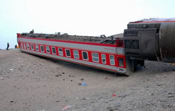
Wind blows train off tracks in Xinjiang, Shanghai Daily 02-28-2007
In two previous blog posts I have discussed the method for calculating cross wind characteristics for train overturning in high winds that is set out in Baker et al (2019). In the first, I used the approach to look at what might be regarded as the “best” shape for trains in overturning terms, and in the second I looked at the methodology itself and tried to understand the quite complex form of the solution of the governing equations. In this post, I will consider the shape of the cross wind characteristics that are predicted by the method and consider how the characteristics change as the form of the lee rail aerodynamic rolling moment characteristic changes.
The method itself is straightforward and is given in the box below taken from a previous blog post. It assumes a simple three mass model of a train under the action of a wind gust and, through a suitable assumption for the form of the rolling moment characteristic allows reasonably simple formulae for the cross wind characteristic to be calculated. The method is considerably simpler than the methodology outlined in “Railway Applications – Aerodynamics, Part 6: Requirements and Test Procedures for Cross Wind Assessment. CEN EN 14067-6:2018” where a multi degree of freedom dynamic model of the train is required, and an artificial wind gust is imposed. I am strongly of the view that the complexity of the latter method is unjustified for two basic reasons. Firstly the use of a highly accurate multi-degree of freedom dynamic model is inappropriate when the input wind gust and aerodynamic characteristics have major uncertainties associated with them and the output is used in very approximate risk calculations; and secondly because the CEN method of specifying the wind gust is theoretically unsound and not representative of a real wind gust as I have argued elsewhere. In any case the methodology I use here has actually been compared against the CEN methodology and can be made to be in good agreement if properly calibrated. I would be the first to admit that a more detailed calibration of the method for a range of “real” effects such as track roughness, turbulence scale, suspension effects etc. is probably required, but its simplicity of use has much to commend it, particularly in helping to understand the physical processes involved.
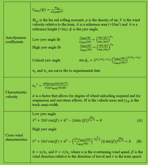
The methodology of Baker et al (2019)
Those points being made, now let us turn to the matter in hand. The methodology starts from a curve fit of the measured or calculated lee rail rolling moment coefficients. The forms chosen are shown in Figure 1 below and effectively requires the specification of four parameters – the lee rail rolling moment coefficient at 30 and 90 degrees yaw, and the exponents of the curve fits n1 and n2, the first in the low yaw angle range, and the second in the high yaw angle range.

Figure 1. Curve fit formats to lee rail rolling moment characteristic
This curve fit then leads to the formulae for CWCs in the two yaw angle ranges given as equations A and B in the box above.. These give the values of normalized overturning wind speed against normalized vehicle speed, as a function of wind direction, the ratio of the lee rail moment coefficients at 90 degrees and 30 degrees and the two exponents. The normalization is through the characteristic velocity which is a function of the train and track characteristics, including the rolling moment coefficient at 30 degrees yaw.
Let us firstly consider the normalized CWCs calculated from this method. Figure 2 shows these for wind directions relative to the train direction of travel from 70 degrees to 110 degrees (where 90 degrees is the pure cross wind case). The lee rail rolling moment coefficients at 30 and 90 degrees are 4 and 6 respectively, and the exponents n1 and n2 are 1.5 and -1, all of which are typical values for a range of trains. From the figure it can be clearly seen that there are two parts of the cross wind characteristic – a low yaw angle range at the higher vehicle speeds, where the normalized overturning wind speed decreases slowly with increases in normalized vehicle speed; and a high yaw angle range for low vehicle speeds, where the normalized wind speed increases above the low yaw angle value, in some cases quite significantly. In general terms the low yaw angle curve is probably of more practical relevance as it corresponds to the normal train operating conditions, at least for high speed trains. Here there can be seen to be little variation of the characteristic with wind angle over the range from 70 to 90 degrees. The minimum value is usually at a wind angle of around 80 degrees, but the minimum is very flat and the values of normalised wind speed for a pure cross wind of 90 degrees are very close to the minimum values.
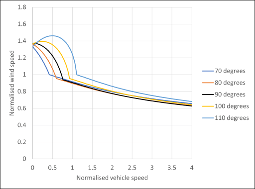
Figure 2 CWC variation with wind direction
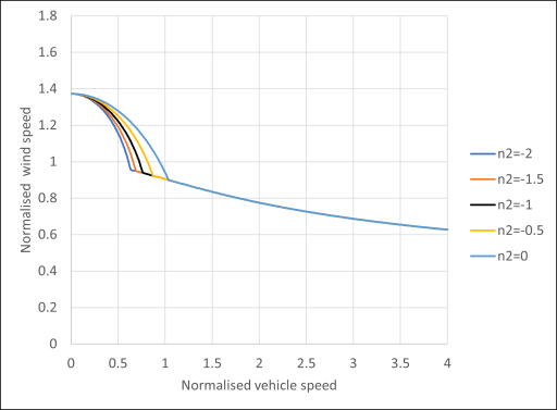
Figure 4 CWC variation with high yaw angle exponent n2
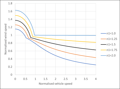
Figure 3 CWC variation with low yaw angle exponent n1
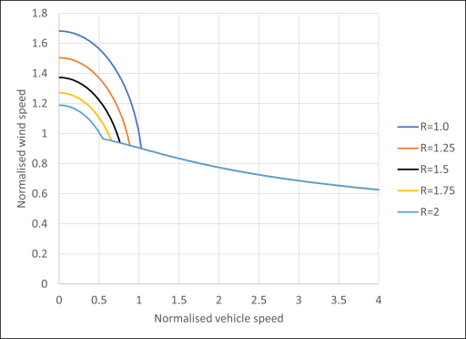
Figure 5 CWC variation with ratio R of lee rail rolling moment coefficients at 90 and 30 degrees yaw
Figures 3 to 5 show the variation of the CWC at a wind direction of 90 degrees for a range of values of the two exponents n1 and n2 and the ratio R of the rolling moment coefficients at 90 and 30 degrees. Firstly the low yaw angle exponent is allowed to vary between 1.0 and 2.0. Earlier work has shown that blunt nosed leading vehicle tend to have a value of n1 of around 1.1 to 1.3, and streamlined leading vehicles have values between from 1.4 and 1.7. There can be seen to be very considerable variation in the CWCs throughout the vehicle speed range as this parameter varies, with the lower values resulting in lower, and thus more critical CWCs (but remember that these are non-dimensional curves – we will deal with the dimensional case below). Variations in the high yaw angel exponent n2 and the ratio of the rolling moment coefficients have a somewhat smaller and more localized effect in the low vehicle speed range only. As to which are the most important parameters, that depends upon the type of train – for high speed trains, the low yaw angle range is critical, but for low speed trains, the yaw angles experienced in practice span the high and low yaw angle ranges so both are important.
To simplify things further, the figures suggest that if the CWCs for the low yaw angle range were used throughout the speed range, then this would be a conservative approach. Figure 6 shows such CWCs for the conditions of figure 3 for a wind direction of 90 degrees, which is very close to the minimum, critical, value, and a range of values of the exponent n1. Note that at zero normalised speed, the normalised wind speed is 1.0 in all cases. By setting the wind direction to 90 degrees, equation A in the box above takes on a very straightforward form, and values of normalised wind speed can be found for any value of normalised vehicle speed for any value of n1, although an iterative solution is required.
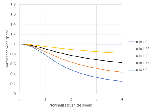
Figure 6. CWCs for all vehicle speeds using low yaw angle formulation only.
All the CWCs presented above have been in a dimensionless form. These can easily be converted to a dimensional form by multiplying the velocities on both axes by the characteristic velocity. This is know to vary between about 30m/s for conventional low speed trains to around 40m/s for high speed trains. The variation in the CWC for 90 degrees wind direction from Figure 2 for these two characteristic velocities is shown in figure 7. The value for 30 m/s lies well below the 40 m/s curve, with very much lower overturning wind speeds at any one vehicle speed. However whilst the high speed train with a characteristic velocity of 40 m/s has a top speed of above 300 km/h, the top speed for the low speed, conventional train with a value of 30 m/s will be around 160 km/h. So a direct comparison at the same speed is not entirely appropriate.
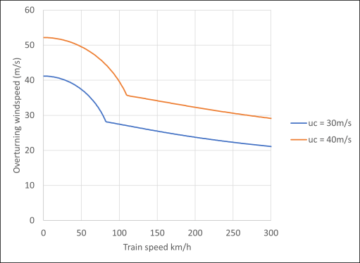
Figure 7 CWCs in dimesnional form
