John Louis Petit – painter and landholder

Preamble

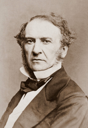
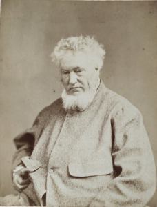
John Louis Petit was a noted landscape painter and critic of ecclesiastical architectural practice in the 19th century. After his death, his work languished in obscurity for many years, but has recently been brought to public attention by the J L Petit Society and is well described on the website of that organisation and elsewhere. He and his sisters painted several hundred pictures of landscapes and churches across England, Europe and beyond. He was able to do so because he was from a wealthy family, descended from Huguenot immigrants to England in 1685. Concerning that wealth the Petit society web site simply says “Petit’s family were moderately wealthy landowners, active in professions, from Staffordshire“. The question then arises as to where the wealth came from that enabled him to pursue his interests through extensive and no doubt expensive, travel, This post unpacks the source and extent of his wealth in a little more depth and leads me to the conclusion that the Petit family were much more than simply “moderately wealthy”. It will be seen that the main source of this wealth seems to have been an estate in the Sedgley / Wolverhampton area, and I will investigate this estate further in a future post.

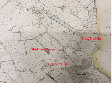
To help the reader in navigating the travels of the Petit family around the Midlands, the map below shows the places mentioned in this post that are in the vicinity of Wolverhampton.

Places named in the text in the vicinity of Wolverhampton

The Petits in England

We begin by considering the first of the Petit family to arrive in England. Lewis Petit (1665-1720), a member of the ancient Norman family of Petit des Etans, fled to England from Caen on the revocation of the Edict of Nantes in 1685, along with many thousands of others. The revocation of this edict led to severe persecution of the protestant Huguenots by Catholics, and many fled the country at that time. He served in the British army as an engineer, rose to the rank of brigadier-general and was appointed lieutenant-governor of Minorca from 1708 to 1713. He was later involved in the suppression of a revolt by Highland clans. More detail can be found in his Wikipedia entry. No doubt he was well rewarded for his services. He had two sons, John Peter Petit and Captain Peter Petit. The former married Sarah, daughter of John Hayes of Wolverhampton, the owner of the Ettingshall Estate near Sedgley, and they occupied the manor of Little Aston from 1743 to the early 1760s. John Hayes died in 1736, and left Ettingshall to his son, another John. This John himself died in 1745 and the estate went to Sarah and her sister, and thus ultimately to John Peter Petit. Ettingshall was a large, originally arable estate, that even at that stage was beginning to be exploited for its coal and ironstone reserves. John Peter also appears to have owned Saredon Hall farm in the village of Shareshill.

John Peter and Sarah’s only son, John Lewis Petit (1736-1780) was educated at Queens College, Cambridge, qualified as a doctor in 1767 and was physician to St. George’s Hospital from 1770 to 1774, and to St. Bartholomew’s from 1774 until his death. He was a Fellow of the Royal Society from 1759 and was clearly regarded as a leader in his profession. He married Katherine Laetitia Serces, the daughter of Rev. James Serces, pastor of the French Church in London. They had three sons John Hayes Petit (1771-1822), Peter Hayes Petit (1773-1809) and Louis Hayes Petit (1774-1849), but clearly lacked imagination in the giving of names. The Ettingshall Estate was inherited in its entirety by John Hayes, with financial provision being made for the other sons. In John Lewis’ will there is the following rather interesting provision.

I desire my body may be opened [for medical science] if the distemper of which I may die shall not have rendered it so loathsome as to endanger the operator and that the sum of ten guineas shall be given to the person who shall perform the operation.

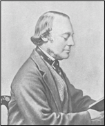
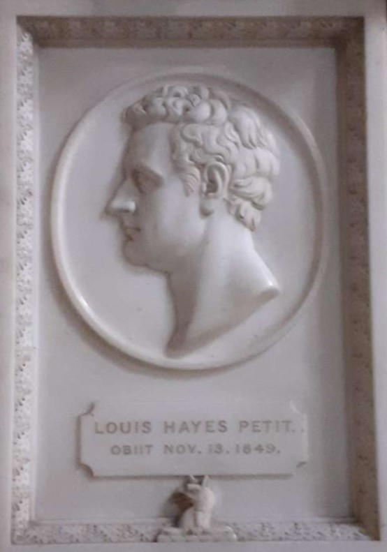
Of the two younger brothers, Peter Hayes was a lieutenant-colonel of the 35th Foot and died at Deal of a wound received at Flushing in Holland during the Napoleonic war. Louis Hayes became a barrister and, from 1827 to 1832, was MP for Ripon. He bought property at Yeading, Middlesex, and a house in Tamworth Street, Lichfield. He also acquired an estate at Merridale in Wolverhampton, not far from Ettingshall, which the sources suggest provided him with income from mineral rights. This cannot however be wholly true as Merridale is to the west of Wolverhampton, and is not in fact on the coal field. It will be seen below that he also possessed land to the east of the town at Bilston, on which there were indeed coal mines, and this was probably the source oft he confusion. After ceasing to be an MP, his remaining years were largely devoted to literary and philanthropic pursuits There is a monument to him at the east end of the north aisle of St Michael’s church in Lichfield.

The Ecclesiastical Petits – John Louis and his father

The eldest of the three brothers, John Hayes Petit (1771-1822) inherited the Ettingshall estate, but also seems to have followed an ecclesiastical career. He was born in Bloomsbury and graduated from Queens College Cambridge with a BA in 1793 and an MA in 1796. He was ordained priest in Chester in 1798 and served a curacy at Ashton under Lyme near Stalybridge in Cheshire.  During his time there he married Harriet Astley of the nearby town of Dukinfield. Harriet was born in 1779 to the painter John Astley (1724-1787) and his third wife Mary Wagstaffe (1760-1832). John Astley had a colourful life, painting portraits of many 18th century notables, arousing strong passions of admiration (mainly in women) or distaste (mainly in men). His first wife was an unknown Irish lady who died in 1749. The second was Penelope Dukinfield Daniel (1722–1762) widow of Sir William Dukinfield Daniel, 3rd baronet, and a daughter of Henry Vernon, former High Sheriff of Staffordshire. John and Penelope were married with some rapidity after she intimated that the original of the portrait he was painting of her would be available if he wished. On Penelope’s death, and the death of his stepdaughter, Astley inherited the substantial Dukinfield and Daniel estates in Cheshire and was able to lead a life of some luxury and idleness thereafter.  Harriett was one of three sisters, known as the Manchester beauties, and her marriage to John Hayes would have brought him both a beautiful wife and a substantial supplement to his already considerable income. 

John Louis Petit, the artist, was John Hayes and Harriet’s eldest son and was born in 1802. For the next few years the family lived a somewhat peripatetic existence. The oldest sister, Harriet Letticia Petit (later Salt) was baptised in Stretton on Dunmore in Warwickshire in 1803. The next two children Mary Ann Petit (1805-) and Peter John Petit (1806-1852), later a Lieutenant Colonel in the 50th Regiment, were baptised at Darfield in Yorkshire. No reason for the Petit family’s presence in these places can be traced. The next two children, Emma Gentile Petit (1808-1893) and Elizabeth Petit (later Haig) (1810-1895) were baptised at Donnington in Shropshire to the north west of Wolverhampton. In January 1811 John Hayes was appointed Stipendary Curate of that parish, and then in February of that year he was appointed as a Perpetual Curate at Shareshill, to the north east of Wolverhampton where he already owned land.  How these posts interacted with each other is not clear. The Vernon family, from whom Harriet was descended, owned Hilton Hall, which was close to Shareshill, and may have been influential in John Hayes obtaining the post.  He held the Perpetual Curacy at Shareshill till his death in 1822. Their next three children were all baptised in Shareshill – Louisa Petit (1813-1842), who died after a “life of uninterrupted suffering, which she bore with a true Christian patience and cheerfulness”; Susannah Petit (1813-1897); and Louis Peter Petit (1816-1838) a barrister at Lincoln’s Inn. Around 1817 John Hayes leased Coton Hall at Alveley in Shropshire from Harry Lancelot Lee, and it was there that their final child, Maria Katherine (later Jelf) (1818-1904) was baptised. Coton Hall was a very substantial property that once belonged to the Lee family. In 1636, Richard Henry Lee emigrated to the US, and the family became rich through the ownership of tobacco plantations with a large slave population, and from whom the US Confederate General Robert E Lee was descended. It would not have been a cheap place to lease. After John Hayes Petit’s death in 1822, Coton Hall was bought by James Foster (1786 -1853), the very successful and wealthy ironmaster and coalmaster of Stourbridge.  John Hayes’ wife Harriet and her unmarried daughters moved to the house in the house in Tamworth St, Lichfield that was owned by her brother-in-law Louis Hayes Petit.

John Louis Petit inherited the Ettingshall estate on the death of his father in 1822, and also inherited the bulk of the estate of his uncle Louis Hayes Petit when the latter died in 1849. In total they formed a very substantial estate in the Wolverhampton area, that was being heavily exploited for coal, iron ore and limestone. He and his sisters also had a less tangible inheritance from his mother and his grandfather – the passion and the ability for painting and sketching. After he graduated from Trinity College in Cambridge in 1825, John firstly pursued an ecclesiastical career being curate at St Michael’s in Lichfield from 1825 to 1828, under the Perpetual Curate Edward Remington, and then curate at Bradfield and Mistley in Essex from 1828 to 1834. During his time at St. Michael’s, the registers tell us he carried out 61 baptisms, 35 weddings and 163 funerals, as well as presumably leading the Sunday worship – a not inconsiderable load. He married Louisa Reid, the daughter of George Reid of Trelawny in Jamaica in 1828. The Reid family derived much of their wealth from slave plantations in Jamaica and the family received considerable compensation for their lost income when slavery was abolished in the 1830s.

The Petit estates in the 1840s

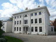
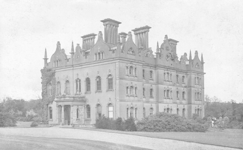
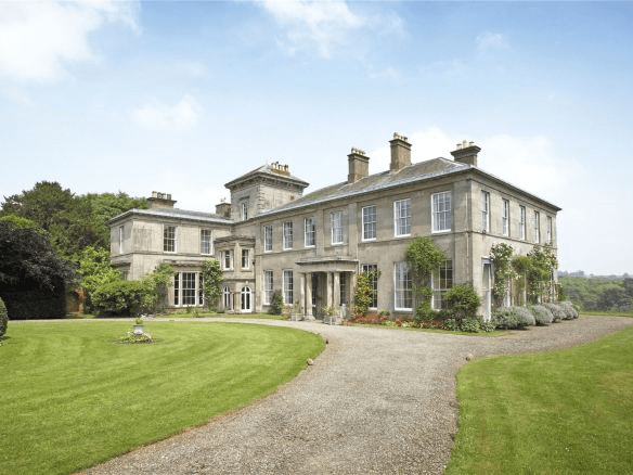
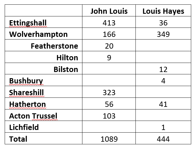
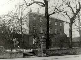
But that is not the end of the matter. Details of the holdings of John Louis and Louis Hayes at the time of the tithe apportionments in the 1840s can be obtained from the tithe maps for Staffordshire. These are shown in the table below. It can be seen that the estates around Ettingshall and Wolverhampton were far from all their holdings. John Louis also held land in Wolverhampton itself, and in Hilton and Featherstone in the north of the town, and in Shareshill, Hatherton and Acton Trussell further to the north. At the time he lived in a house at Shifnal in Shropshire. Louis Hayes, as well as the land in Wolverhanpton also had holdings in the vicinity of the town at Sedgley and Bilston, as well as at Bushbury and Hatherton to the north. He also held the property in Lichfield where Harriet and her daughters lived. A photograph of this rather imposing property, Redcourt House, is shown below. It was situated on Tamworth Street downhill from the junction with George Lane, and its grounds extended a considerable distance behind it between what was then Back Lane and Frog Lane. In total John Louis held nearly 1100 acres and Louis Hayes nearly 450. This would have put them amongst the major landowners in the Midlands. Whilst the lands around Wolverhampton and Sedgley can be explained as an expansion of the Ettingshall and Merridale estates and the family had held land in Shareshill for several generations, there is no obvious reason why the lands at Bushbury, Hatherton and Acton Trussell came into their possession. One possible reason might be that these were holdings of Penelope Dukinfield Daniel through her descent from the Vernon family who held land in that part of Staffordshire. This might explain why John Hayes and Harriet made their home at Shareshill and the former became the Perpetual Curate in the parish.

Petit land holdings in Staffordshire in the 1840s. Numbers indicate the area in acres
Redcourt House

But there is yet more. In Staffordshire Archives, there is an index record that states ” Abstract of title of late John Louis Petit in Staffordshire and Hereford, Radnor and Brecknock “. It would appear that the property in Hereford was the estate of Bollitree Castle, a large house with mock fortifications, with Louis Hayes owned at the time of his death. I have not been able to identify any properties in Radnor and Brecknock.

Epilogue

So to return to my original query, it would seem that the Petit wealth derived in the main from a series of very advantageous marriages – and in particular those between John Peter Petit and Sarah Hayes, which brought the Ettingshall estate into their positions. This estate will be the subject of a further blog post. In addition the family were clearly successful in the professions in which they worked as a result of their very considerable talents. One point that I still find difficult to understand is why John Hayes and John Louis pursued ecclesiastical careers – the clergy stipends were almost certainly of little significance in terms of their overall wealth. Perhaps the holding of a clergy post gave a degree of respectability to a life of leisure. At any rate, John Louis gave up his post in Essex in 1834 and from the mid-1830s onwards he devoted his time to his painting and architectural criticism, and his story is told elsewhere.

The calculation of train overturning risk – what type of wind tunnel tests should be used?

A Mark 3 coach – the GB benchmark vehicle

When considering the effect of crosswinds on a new train, an obvious first step is to obtain data on the aerodynamic force and moment coefficients, usually through the use of wind tunnel tests, with the forces and moment coefficients being measured for a range of yaw (wind) angles from 0 to 90 degrees. This process however is not quite as straightforward as it sounds. The conventional approach is to use static models in a low turbulence wind tunnel. This approach of course models neither the relative motion between the train and the ground, nor the effects of atmospheric turbulence. It does however have the merits of simplicity and convenience. The conventional argument often used to justify this approach is that for high-speed trains, the relative motion between the train and the wind leads to the train experiencing low levels of turbulence. Whilst this is the case to some extent, it is not a wholly adequate argument. Figure 1, from Train Aerodynamics – Fundamentals and Applications (TAFA), shows how the turbulence length scale, turbulence intensity and velocity shear relative to the train vary with train speed for a 90 degree cross wind. Values are given as ratios of the values when the train is stationary. It can be seen that even at 400 km/h, the train still experiences a turbulence intensity of around 30% of its stationary value, which one might expect to have a not insignificant effect on the flow around the train,.

Figure 1 Variation of relative values of turbulence intensity (black), turbulence length scale (red) and shear (green) with train speed for a 90 degree cross wind (from TAFA)

An alternative approach would be to use a wind tunnel simulation of the atmospheric boundary layer in which to measure the train forces and moments. This of course is only really applicable to stationary trains. On the basis of figure 1, I argued in TAFA that low turbulence wind tunnel tests would be best for train speeds greater than 200 km/h and atmospheric boundary layer tests would be best for train speeds below that value – but that of course represents rather a messy compromise. And both methods fail to address the issue of train / ground relative motion.

So what are the alternatives? The first might be thought to be the use of CFD to properly model both atmospheric effects and train / ground motion. However, the simulation of a realistic scenario requires complex CFD methodologies (usually DDES) with very complex domain boundaries that include the specification of atmospheric turbulence. The calculation of the flow field for just one yaw angle takes several weeks on supercomputer systems, and in reality CFD calculations of this type tend to mirror the low turbulence wind tunnel tests.

In physical model terms, two alternatives present themselves. The first is the measurement of cross wind forces and moments on a moving model rig such as the TRAIN Rig owned by the University of Birmingham.  Again, the experimental issues are formidable. The use of force balances within moving model rigs is not straightforward, and measurements of this type are usually made through the measurement of surface pressures with internal transducers, which because of transducer size and the need to carry out multiple runs to obtains stable average pressures requires multiple runs, with different pressure positions at any one yaw angle – a very tedious and complex process. An alternative would be to carry out conventional wind tunnel tests, but with a range of different turbulence simulations, each simulation being valid for one train speed only. The thought of such tests is enough to make wind tunnel operators consign it to the rubbish bin without much hesitation.

But the issue is important. Figure 2 shows three different sets of lee rail rolling moment coefficients for the Mark 3 coach, the GB benchmark vehicle that has run on exposed lines for many decades without incident. The three sets of coefficients are obtained from low turbulence wind tunnel tests; tests with an atmospheric boundary layer simulation with the coefficients formed from the mean values of measured forces and velocities; and those obtained from similar tests but with the coefficients formed from one-second peak values of forces and velocities (from Measurements of the cross wind forces on trains). The atmospheric boundary layer results are shown together with corresponding full scale results from field measurements on a real train. There can be seen to be significant differences between the three curves, particularly in the low yaw angle range which is important at high train speeds, with the low turbulence values being significantly above the atmospheric boundary layer values and the peak values being below the mean ones. If these coefficients are used to obtain cross wind characteristics (CWCs), which are plots of accident windspeed against vehicle speed, as outlined in another post and in TAFA chapter 11 and in a recent blog post, then the differences in acceptable windspeeds can be seen to be significant, particularly in the speed range around 200 km/h – see figure 3. Note that this plot shows train speeds of up to 400 km/h, which is wholly unrealistic for the Mark 3 coach – and certainly I wouldn’t care to be in one travelling at that speed! – but serves to illustrate the lack of agreement between the CWCs calculated using different moment coefficients. The difference in CWCs can be expected to make a significant difference to the calculation of accident risk, or to any operational restrictions that might be imposed, with the low turbulence results giving higher risk values and more severe restrictions.

Figure 2. Lee rail rolling moment coefficients for Mark 3 coach

Figure 3 Crosswind characteristics for Mark 3 coach

I have to admit this is a problem that I have been mulling over on and off for many years (which gives a rather sad picture of the life I lead I fear). My thoughts have been basically around the idea of how to obtain representative force coefficients to allow for the major effect of atmospheric turbulence at low train speeds and the much smaller effect at high speeds, perhaps by some interpolation of the low and high turbulence coefficients. This is not simple however, as there is no direct correspondence between variation of these coefficients with yaw angle and variation with train speed.

But there is perhaps another way – and that is to consider not the force and moment coefficients, but rather the CWCs shown in figure 3. It seems reasonable to me to assume that the most representative CWC would lie somewhere between the low and high turbulence characteristics, lying close to the ABL curve at low train speeds, and close to the low turbulence curves at high train speed. Thus figure 4 shows the CWCs formed from giving a variable weighting to the low and high turbulence curves at different train speeds, with a 100% weighting given to the low turbulence curves at a train speed of 0 km/h, and a 0% weighting at a train speed of 400 km/h, with a linear variation in between. More sophisticated weighting variations could be considered, but this approach is adequate for illustrative purposes. The two curves of figure 4 are for the interpolation of the CWCs calculated from the mean and peak coefficients with those obtained from the low turbulence coefficients. It can be seen that this approach significantly raises the CWCs in the mid speed range from the low speed values and will thus result in substantial risk reduction.

Figure 4. Interpolated cross wind characteristics

Up to now, I have referred to potential risk reductions in rather broad terms. It is however possible to put some numbers to these statements. Table 1 shows the accident wind speed at a train speed of 200 km/h for each of the above CWCs and the associated risk at the reference site as defined in my earlier post. For the original CWCs derived from the ABL coefficients, , the risks is of the order of 10-7 to 10-8, but for the CWC derived from the low turbulence conditions, the risk approaches 10-5 – almost two orders of magnitude greater. Whilst the absolute values of risk are quite arbitrary, it is clear that the use of the low turbulence characteristic would lead to a much more pessimistic (and perhaps unrealistic) risk assessment, and lower than necessary wind speed restrictions. The interpolated CWCs give values of risk of ca little less than 10-6, roughly midway between the atmospheric boundary layer and low turbulence values.

Table 1. Accident windspeeds and risk values for Mark 3 coach at a train speed of 200 km/h

So to conclude, the method outlined above gives a potentially realistic way of solving the problem of what type of wind tunnel test to use for train cross wind risk assessment. It requires two sets of wind tunnel experiments, one with low turbulence and one with an atmospheric boundary layer simulation, which is a more complex methodology than at present, but does not require extremely complex wind tunnel or CFD trials. The method results in lower values of calculated risk than would be the case using conventionally derived CWCs, and higher values of accident wind speeds.

International Wind Engineering seminars 2020/21 – some reflections

A Japanese version of this post can be found here

Between October 2020 and March 2021, I organised a series of six International Wind Engineering Seminars, through the University of Birmingham, my employer before I retired. These were sponsored by the International Association of Wind Engineering (IAWE) and delivered via Zoom. On the web page for this seminar series, I give the justification for organising it as follows.

“Because of the Covid19 pandemic, opportunities for the international wind engineering community to meet physically have been very much restricted and are likely to remain so for at least the next year. To enable the community to continue to interact with each other, at least in a virtual way, the University of Birmingham is organizing a series of six seminars via Zoom from October 2020 to March 2021.”

In this post, I want to reflect on how these seminars were delivered and received, what lessons might be learnt, and ask some questions concerning the future.

Each seminar consisted of a main speaker, followed by either a panel discussion or between two and four shorter presentations. The dates and topics are given in table 1. As these seminars were set up in some haste in August / September 2020, I mainly called upon my circle of contacts to be the main speakers at the events, and they suggested other speakers or panel members. I am indebted to all the speakers for taking part and spending considerable time in preparation. The nature of the delivery and follow up evolved over the course of the series. After the first seminar it became clear that I could not both chair the sessions and organise the questions in Chat to put to the speakers. Thus, from seminars 2 to 6, I was assisted by Grace Yan from Missouri who collated all the questions that were put on Chat and forwarded them to me to put to the speakers. Her help was hugely appreciated. For seminars 3, 4 and 6 the presenters and panelists were also asked to provide written answers to questions, and these were posted on the web pages that were for each of the seminars. All the presentations (and for seminars 5 and 6 the questions and answers) were recorded using the Zoom Record function and these recordings were place on my YouTube site and linked to the appropriate page. These pages also included talk abstracts and speaker biographies. After the third seminar I realised that YouTube could not be accessed from all parts of the world, so a link to the Zoom cloud versions was also given. From seminar 4 onwards, these could also be downloaded as required. The time chosen for the seminars (after the first) was 12.00 UK time, this being the best compromise for most time zones, with the exception of the west coast of the America and Australasia. I tried to institute a separate Q and A session for these time zones a day or so after the seminar, but there was insufficient take up to make it worthwhile. Thus the whole process was a considerable learning experience for me.

Table 1 Seminar dates, titles and speakers

It must be mentioned at this point that the third seminar occurred shortly after the death of Prof Giovanni Solari, who was instrumental in the setting up of the IAWE, and the speaker, Prof Kareem, paid tribute to him in his talk.

UniGe Giovanni Solari
Prof. Giovanni Solari

Table 2 shows the bare statistics for the seminars. The size of the distribution list for publicity grew through the series from the original 688 of the mailing list for the abortive BBAA conference to 1525 for seminar 6.  By seminar 3 the size of the list became so large that my e mail account was temporarily stopped as it was thought it had been hacked and was sending out spam. Thereafter I sent the information around in smaller batches. The number of registrants varied between 279 and 616, although only around 50 to 70% of these actually connected. The number of video views was also encouraging although again one must interpret these numbers cautiously as only around 20 to 30% of the views were for more than a few minutes. Note that these statistics are up to March 14th 2021 only, and as the views continued for several months after each seminar, the number of video views for the 2021 seminars will not be the final values.

Table 2 Seminar statistics (up to March 14th 2021)

Table 3 shows a breakdown of the views of the seminar web pages by month (which includes links to the videos). As expected these peak just before and just after the seminar, but all the seminars attract a significant number of views for a number of months after the event, which suggest that the subject matter is of ongoing interest. Again, note that this date only extends to the middle of March 2021,and a significant number of views could be expected for the later seminars after this date.

Table 3 Views of seminar web pages (up to March 15th 2021)

Table 4 shows the location of those who registered, as far as could be judged from email addresses. The generic .com address contains registrants from a wide variety of countries, and this rather skews the results. Nonetheless, it can be seen that whilst those countries where wind engineering is well established are well represented, a very wide range of countries was represented overall.

Table 4 Locations of registrants

Thus the numbers suggest that there was a significant number of wind engineers around the world who appreciated the seminar series and found them useful, and indeed that is what has been suggested by the informal feedback I have received. Again, caution is required to avoid over interpretation – the level of engagement with online seminars is likely to be much less than with in person presentations – I for one tend to do things such as checking my e mail / cricket scores when attending such virtual events – but not when I am chairing of course! But broadly the seminar series seems to have met a need. But there are needs it hasn’t addressed, for example the inclusion of a social aspect for informal discussion and the inclusion of young researchers in a meaningful way etc. To address this sort of issue, other formats can be envisaged – for example I can think of the following.

  • Specific discussion topics could be set, and potential attendees asked to submit short abstracts of a two minute, two slide talk, from which a balanced group of young and established researchers could be selected for a series of short presentations and a more relaxed discussion. These could be recorded and put on-line for all to see.
  • Interviews (by me or others) of a range of wind engineers, talking about their careers, their successes and failures etc., which could again be recorded and put on-line.
  • The use of a platform such as Gather Town, which seems to allow for multiple individual conversations within a group structure and could be used for, say, virtual poster sessions (but note I have never used this, although on the face of things it seems potentially useful.)

And there are no doubt other possibilities. The question then arises as to what should happen next. I don’t intend to organise any more such seminars till September at least – amongst other things I wish to watch a number of cricket matches rather than just checking the scores, and to re-acquaint myself with a number of heritage railways in Wales. So, I put the following questions to the wind engineering community.

  • Should something similar be organised for next winter as I suspect international travel won’t resume in any real sense until Summer 2022 at best? Note that I am not necessarily implying that should something felt to be necessary, then I would be the one to organise it!
  • If so, what should the format be – just one speaker, or more than one speaker, or something completely different?
  • Are there any suggestions for topics and speakers?
  • Are there any other suggestions for possible related activities, such as I mention above.

There is also a larger question of course about the future of the four year cycle of Wind Engineering conferences and whether such a cycle is still sustainable – see for example the initiative of Glasgow University which is urging academics to reduce overseas travel as part of the greening of its activities. But that is a discussion for others to have within the IAWE committee.

Please make any comments in the comment box attached to this post, or, if you wish, email me directly on bakercj54@gmail.com. Thanks in advance.

Kingswinford Landowners and Industrialists in the 19th Century – some surprising names

Preamble

As outlined in Kingswinford Manor and Parish, the Fowler Maps of 1822 and 1840 gave a great deal of information concerning the landowners and occupiers of the parish at those times. In the main most of the landowners were quite local, with the major ones being the Earl of Dudley’s Estate and John Hodgetts-Foley. However, a few surprising names of landowners and industrialists crop up – those who have some sort of national profile outside the immediate area of the Black Country. In this short post, I briefly consider three of these – Jonathan Stokes, Horace St Paul and Stephen Glynn and his fellow owner of Oak Farm Iron Works.

Jonathan Stokes

Jonathan Stokes (1755-1831) was an Edinburgh trained doctor, and, from 1782 to 1788 was a member of the Lunar Society, one of the intellectual driving forces of the period whose members included Matthew Boulton and Erasmus Darwin. He is remembered for his work, in collaboration with others, on the uses of digitalis. His parents were Rebecca and Jonathan Stokes, “Gentleman of Worcester”. Many of the sources say he was born in Chesterfield, although this has recently been shown to be untrue and his birth in Worcester has been established. He had a practice in Stourbridge for a number of years from 1782 to 1785. His membership of the Lunar Society ended following fierce arguments with his colleague William Withering over authorship of a book. He married Ann Rogers, a “minor poet” at Dronfield in 1784. The marriage was four months after the birth of Jonathan and Ann’s first child John Rogers Stokes (1784 – 1818), and Jonathan does not appear on the baptismal record. Their second son John Allen Stokes was born in Shrewsbury in 1786, being baptized in a Presbyterian Meeting House. They had other children. Of particular note are Anna Honora Seward Stokes (1791-1792) and Honora Anna Seward Stokes (b1794) both named after the poet Anna Seward, ‘the Swan of Lichfield” with whom they were close friends. 

In 1788, Rebecca Stokes, at that point a widow, was involved in the sale of a plot of land on which the Red House Glassworks in Wordsley was built. She clearly owned other properties in the area, and in 1822 Jonathan, as her heir, held a number of scattered plots across the parish, mainly concentrated in the area enclosed by the Ashwood Hay Enclosure Act of 1776 and the Wordsley and Brettell Lane areas. These amounted to around 200 acres in total of mainly arable land, with a few domestic properties. In 1840, these were in the hands of his son John Allen Stokes. How the Stokes came into the ownership of such extensive lands in Kingswinford is not clear. One possible route comes from a recorded marriage in 1781 between Nancy Freeman, one of the illegitimate children of John Keeling, the agent and steward of the Dudley estate who owned significant property in the area, and one William Stokes. Links with either Jonathan however cannot be demonstrated, so this must be conjectural. Keeling did however provide generously for his illegitimate offspring, and this might be another example of his provision.

Horace St Paul

Sir Horace St Paul (1775-1840) was a career soldier who became MP for Bridport from 1812-1832 and was created a Baronet in 1813. His father was

“a Northumbrian gentleman driven into exile after killing a man in a duel and was a soldier of fortune in the Seven Years’ War, who returned to England with an Austrian title and a royal pardon, subsequently distinguishing himself in diplomacy, before retiring to his ancestral home.”

The St Paul crest

The Austrian title was as a Count of the Holy Roman Empire, which his son inherited, the most impressive of all the titles of Kingswinford landowners. In 1822 he owned around 30 acres of arable land in the Kingsley Road / Mount Pleasant area of Kingswinford, to the east of Ridgehill Wood, and almost certainly came into his possession through his marriage in 1803 to Anna Maria, the natural daughter of John, 2nd Viscount Dudley whose forebears were granted the lands at the Ashwood Enclosure in 1776. Unfortunately however, the current residents of Kingsley Road and Mount Pleasant share the defining characteristics of their former owner’s title – they are neither Holy, nor Roman, nor in any sense, Imperial.

Stephen Glynne and the Oak Farm Iron works

The Glynne Baronetcy dates back to 1661, with its main estate at Hawarden in Flintshire. The 8th Baronet, Sir Stephen Glynne (1780 to 1815)  married Mary Griffin, daughter of Lord Braybrooke. After his early death, he was succeeded by his son Sir Stephen Richard Glynne, the 9th Baronet (1807-1874). He was a Conservative Party politician and is principally remembered as aa noted antiquary and student of British church architecture and writer of a treatise entitled “Notes on the Older Churches in the Four Welsh Dioceses”.

The Glynne family were also the owners of around 100 acres of land around Oak Farm in the north of Kingswinford parish. In 1822, these are in the possession of “Lady Glynne”, presumably the widowed Mary, as the younger Stephen was still a child. At this time these lands were wholly agricultural. In 1840, the same area was owned by the Oak Farm Colliery Company .The Tithe Allocation records the owners as Thomas Bagnall, James Boydell, Baronet Sir Stephen Glynn, John Hignett, William Hignett and Charles Townshend. By this time the lands were a mixture of arable, collieries, brickworks and the major industrial concern of the Oak Farm Iron Works. The latter was founded in 1835 by  Sir Stephen Glynne, Lord Lyttleton, W. E. Gladstone and James Boydell. Gladstone, the future Chancellor and Prime Minister, and Lyttelton had both married sisters of Stephen Glynne.

The Oak Farm works suffered major financial issues, and the company failed in 1848. These events that led to this are set out at some length in the Grace’s Guide entry for Oak Farm. There are conflicting views as to the causes of the financial difficulties – with James Boydell as Managing Partner described as either as being massively over optimistic and extravagent, or as being unsupported by the other owners during difficult time. One source writes

“…the brothers-in-law (Glynne, Lyttleton and Gladstone) appear to have suffered enormous financial losses, but the experience gained by W E Gladstone in dealing with the company’s debt was said to have stood him in good stead when he became Chancellor of the Exchequer…”

Thus the affairs of Kingswinford parish seem to have had a long lasting effect on the country as a whole! There is of course also a legacy of the Glynne family in Kingswinford itself with the name preserved in the Glynne Arms – the Crooked House.

Finally it is worth just saying a little more about James Boydell. He came from Denbigh in north Wales and was a prolific inventor and patent holder. He is best remembered for his “endless railway” system, From Grace’s Guide again.

“….. the ‘endless railway’ system, applicable to traction engines and trailers. A number of flat feet were attached to the outside of a traction engine’s wheels. They were hinged in such a way that as the wheel revolved each succeeding foot would lie flat in contact with the ground, thus spreading the weight of the engine, and allowing the wheels to roll on the plates. The idea was that this arrangement would be more efficient for road-haulage engines, enabling them to deal with poor road surfaces…..”

File:Im1896EnV82-p138.jpg
The Endless Railway System

He seems to have invented the tank!

Kingswinford families – the Corbyns, the Bendys and the Hodgetts. Part 3 – The Hodgetts of Shut End and Prestwood

Part 1 of this blog can be found here, and part 2 here.

If success can be measured in terms of social enhancement, the Hodgetts family is perhaps the most successful family in Kingswinford history. The early Hodgetts shown in the tree below all came from the Kingswinford / Shut End area and John Hodgetts (1550-1630) and John Hodgetts (1595-1634) are both described as yeomen farmers in their wills – see Kim Simmonds Family Genealogy, 2019, which also gives sources for these genealogies. Where their land was in relation to that of the Corbyns at Corbyn’s Hall and the Bendys at Shut End is not clear, but by the 18th and 19th centuries the Hodgetts held large tracts of land in Kingswinford and elsewhere, had married into one of the new aristocratic industrialist families, served as MPs for various places in the locality and lived in Prestwood House – the largest of the gentry houses in the Kingswinford area.

The Hodgetts Tree. Shaded boxes show links with other trees in KMAP

In the 15th and 16th centuries however the Hodgetts’ horizons were more limited. In the 1490s, Edward Sutton (1460-1531), 2nd Baron Dudley, leased land in the Russell’s Hall area to “Thomas Hodgetts of Swinford”, almost certainly the Thomas Hodgetts (1465-1532) at the top of the Hodgetts tree. Similarly, in 1526, Edward leased the “erbage, justment and pannage, etc. of the New Park at Pensnett Chase”, to Thomas’ son John Hodgetts (1495-). It is also possible Henry and William Hodgetts of Sedgley, who between 1610 and 1650 were custodians of the bones of St Chad after they had been removed from Lichfield Cathedral by Arthur Dudley, Edward’s nephew, in 1538, were also related to the Kingswinford Hodgetts.

The recurring generations of John Hodgetts tended to marry the daughters of local gentry – for example Margaret Paston (-1675), the daughter of the Rector Nicholas Paston; or to Hannah Bague (1652-1712), the daughter of George Bague and granddaughter of Gload de Bague, the glassmaker family from Lorraine, and major industrialists in the Wordsley / Brettell Lane area.  John Hodgetts (1650-1716) was Agent of the Dudley Estate in the early years of the 18th century. His daughter, Patience Hodgetts (1685-1772), married Richard Keeling(e) (1677-), who was also the Agent of the Dudley Estate.  Richard and Patience’s niece Ann Hodgetts (1709-1766), daughter of Thomas Hodgetts (1678-1740), Rector of Kingswinford and vicar of Press in north Shropshire, married their son John (1713-1783) who was, once again, the Dudley Estate Agent.

It was John Hodgetts (1650-1716) who purchased the Corbyn’s Hall estate on the death of the last male Corbyn in around 1688 and took up residence there until he sold it on early in the next century. His grandson, John Hodgetts (1698-1742) married Mary Bendy, the co-heiress of William Bendy and through her he inherited at least a significant proportion of the Bendys Shut End estate. This John became High Sherriff of Staffordshire in 1737 and was himself the Agent of the Dudley Estate.

Their son, John Hodgetts (1721-1789) took the major step in the families climb up the social ladder by marrying Elizabeth Foley (1707-1759). The Foleys were descended from Richard Foley, a Stourbridge nailer from the 16th century, who had become extremely wealthy as a result of a successful marketing of his products and were heavily involved in iron production around the Midlands. Richard’s grandson, Thomas (1617-1677) built Witley Court in the Malverns and was High Sherriff of Worcestershire in 1656. He was the first of the family with political ambitions and served as an MP for Worcestershire and Bewdley. Elizabeth was Thomas’s great-granddaughter through his son Philip (1648-1716), with this branch of the family being based at Prestwood at the western edge of Kingswinford parish. John Hodgetts (1721-1789) was, like his father, High Sherriff of Staffordshire in 1765, and seems to have taken up residence at Prestwood on his marriage. Shut End House at this time (approx. 1760 to 1780) seems to have been the residence of Commander John Becher, RN, but the actual ownership is not clear.

In 1790, the daughter of John and Elizabeth, Eliza Maria Foley Hodgetts (1759-), married a cousin from another branch of the Foley family, Edward Foley (1747-1803). This was Edward’s second marriage, with the first having been annulled (presumably by Act of Parliament) but no reason for this can be found. He was the proprietor of the Stoke Edith estate in Herefordshire, and the marriage settlement specified that Eliza and Edward’s oldest child, Edward Thomas Foley (1791-1847) should inherit Stoke Edith, and their second son, John Hodgetts Hodgetts Foley (1797-1861), should inherit the Prestwood estate. It was this John who, through his major land ownership in the Kingswinford area, was to play such a major role in its industrialization. He was the Whig MP for Droitwich from 1822 to 1834 and for East Worcestershire from 1847 to 1861. His rather odd name was the result of formalizing Hodgetts as part of the surname by royal license in 1821. He was married to Charlotte Margaret Gage, granddaughter of General Thomas Gage, who commanded the British armies in the early stages of the US War of Independence. By the time of the Fowler Maps of 1822 and 1840, he held the largest block of land in the manor after that of the Earl of Dudley – 381 ha in 1822 and 266 ha in 1840. His properties in 1822 were built around the old Hodgetts estates in Shut End, the former lands of the Bendy family in Shut End and Holbeach, and the Foley inheritance at Prestwood. He had also gained significant land from the Enclosure Acts in the Ashwood enclosure, largely extending his Prestwood holdings, and also some land in the Pensnett area following the enclosure of the Chase. Foley himself lived at Prestwood, while Shut End Hall was leased to Thomas Dudley (1749-1829), part of the Dudley family with extensive inter-generational marriage links with the Hodgetts, Keelings and others. The land around Prestwood was leased out as two farms – North Farm of 96 ha farmed by Robert Roper, and South Farm 0f 73.5 ha farmed by John Beddard.  By 1840 Foley’s total ownership in the parish had decreased somewhat, through the sale of the Shut End Estate to James Foster. Foster was a prominent local Ironmaster from Stourbridge, who owned the firm John Bradley and Co., and was also partner in Foster, Rastrick and Co. He radically changed the nature of the Shut End Estate, with the demolition of the Hall, and the building of the Shut End Blast Furnaces in the grounds, together with associated coal and iron stone mines. He was also instrumental in the building of the Kingswinford Railway and the Stourbridge Extension canal to serve these works. Around Prestwood both farms were by this time leased to John Beddard (157 ha in total).

Prestwood

The Hodgetts tree shows the extensive connections made by marriage with other local families over the course of the centuries. The Bendy, Foley and Bague families have already been mentioned but we also see marriages to the Keeling, Addenbrooke and Brettell families. The Keelings family were holders of major blocks of land in the Kingswinford area in the seventeenth and eighteenth centuries, and both Richard (1677-) and John (1713-1783) served as agents and stewards for the Dudley Estate. John was the last of the line and after his death his properties were held by trustees for 40 or more years, before being divided amongst the descendants of his mainly illegitimate children.

The Addenbrooke family members were also major landowners in the Kingswinford area. Jeremiah Addenbrooke (1701-1773) married Hannah Hodgetts in 1726, one of the two daughters of Thomas Hodgetts (1678-1740), the vicar of Kingswinford mentioned above. The most famous of the Addenbrooke family, John Addenbrooke, the student and fellow of St Catharine’s Hall in Cambridge who founded the Cambridge hospital was the son of Samuel Addenbrooke (1642-1710) shown in the tree, but, despite his fame, he is not a major character in Kingswinford history.

The other family that occurs in the Hodgetts tree is that of the Brettells, who were by marriage related to the Bague and Addenbrooke families. They are clearly an old established Kingswinford family, important enough to have an important thoroughfare name after them in Brettell Lane but are quite hard to pin down. Whilst there are many occurrences of the name Brettell in the marriage and (particularly) death registers, there are very few baptismal entries that would enable their descent to be determined. This is presumably because they were non-conformists of some form (and their association with the Bague family supports this assumption), and the baptismal lists of whatever chapels they might have attended have not survived.

Although KMAP does not take the history of the Hodgetts beyond about 1850, the family contend to reside at Prestwood. John Hodgetts Foley’s son was Henry John Wentworth Hodgetts -Foley (1828-1894), who was also an MP representing South Staffordshire from 1857–1868. He married Jane Frances Anne Vivian, the daughter of the first Lord Vivian. Their son Paul Henry Foley (19 March 1857 –21 January 1928) inherited the Stoke Edith estate, the other portion of the Foley / Hodgetts estate from his great aunt in 1900.  Paul Foley briefly played first class cricket for MCC and was influential in the formation of the Minor Counties Championship and was the leading figure in the transformation of Worcestershire CCC from an amateur side to one that won the Minor County Championship on several occasions and gained entry to the County Championship itself in 1899. He was also responsible for the purchase of the Worcestershire New Road ground and the construction of the pavilion there. With these most commendable of activities, Paul more than atoned for whatever may have been the sins of the ambitious Hodgetts in their rise up the social ladder.

Kingswinford families – the Corbyns, the Bendys and the Hodgetts. Part 2 – The Bendys of Shut End and Holbeache

Extract from the Fowler Map of 1822

In Part 1 of this post we looked at the first of the three Kingswinford families that were well represented in the historical records of the 16th and 17th centuries – the Corbyns of Corbyn’s Hall. Socially these were probably regarded as minor aristocracy. In this post we will consider the second of these families – the Bendys of Shut End – who came from less exalted stock.

A simplified Bendy family tree is shown above. This is still quite complex and shows marriage links with a number of local families. Much of this information is taken from the excellent Morgan web site, which includes information from a range of wills and other sources.

The Bendy Tree (shaded cells indicate links with other trees in KMAP)

The early members of the tree were associated with the general Kingswinford area, with Richard Bendy (-1592) and Elizabeth Jones being married in Dudley, and Elizabeth being buried in Kingswinford. Their son William (1560-1598) was married to Elizabeth Brookes in Worfield, over the county border in Shropshire. They had just one child, another William (1593-1657). After the death of the elder William in 1598, Elizabeth probably married again to Richard Lee in Alveley, again in Shropshire, and thus, with her son, would have lived on the Lee estate at Coton Hall. The younger William married Mary Barnesley from Trysull on the Staffordshire / Shropshire border, and their eldest son (inevitably another William) was born there in 1620.

William Bendy (1593-1657), although referred to as a yeoman (farmer) in his will, was clearly well connected, perhaps because he was bought up in Coton Hall. He seems to have been based in the Shut End area either at Shut End House or Shut End Hall The name of Shut End is no longer in common usage. It referred to the region around the Dudley Kingswinford Turnpike Road in the High Oak / Tansey Green area. Shut End Hall was to the north of the road, and Shut End house to the south, close to Corbyn’s Hall.  After the thwarting of the Gunpowder plot, the family come into possession of Holbeach House, the home of one of the conspirators, Stephen Lyttleton. William Bendy (1593-1657) would have been a minor at the time of the Gunpowder plot so could not have acquired Holbeach House directly. His elder son William (1620-1684) took his BA at New Hall Oxford in 1637, and at the very young age of 18 was admitted to Lincoln’s Inn in London.  Two other sons Nicholas and Edward (not shown in the tree) also worked in London, whilst another, Samuel, was a Fellow of St Johns College, Cambridge.  The elder William’s chief claim to fame was as a member of the Committee of Stafford from 1643 to 1645, whose task was to suitably dispose of the Royalist property in the county for the Parliamentary forces. As such he would have found himself, as happened very frequently in that period, at odds with other families in the locality – and in particular his neighbours at Corbyn’s Hall.

William Bendy (1620-1684) married Dorothy Lee, daughter of Lancelot Lee of Alveley, thus making further connections with that influential family. The executors of his will were named as his brother-in-law, Lancelot Lee, and his uncle Richard Brettell. William and Dorothy had a number of children, the oldest of which was William (1653-1725). This William married twice, his first wife being Margaret Hoo, daughter of John Hoo of Bradley, by whom he had two girls, Margaret and Mary. His second wife was Mary, who bore him a number of children after Margaret’s death in around 1695, including William (1700-1782).

The sisters Margaret and Mary are referred to in various documents as William’s heirs, and it would seem they inherited most of the estate. Both married – Margaret to John Dolman, Vicar of Aldridge, and Mary to John Hodgetts of Shut End (1698-1741), the grandson of the John Hodgetts who purchased the Corbyn’s Hall estate. In documents from 1752, Mary Hodgetts and her son John are both referred to as living at Shut End and Margaret Dolman and her daughter are living at the Cathedral Close in Lichfield. Both seem to have some sort of interest in Holbeach House. The physical relationship of the properties of the Hodgetts and the Bendys around 1700 to 1750 is not at all clear and the sources are confused.   On balance it would seem best to assume that, in the first half of the eighteenth century, Shut End House (to the south of the Turnpike Road near Corbyn’s Hall) was the ancestral home of the Hodgetts, and Shut End Hall (to the north of the Turnpike Road) and Holbeach House were both in the possession of the Bendys. Shut End Hall was obviously quite a grand dwelling and the extract from the Fowler Map of 1822 above, shows a long avenue of trees extending own into Kingswinford village. By 1822, it was owned by the Hodgetts (or rather the Hodgetts-Foleys at that time) , although they did not live there, so that property clearly passed to them in some way.

William Bendy (1700-1782) lived in the “New House”, situated on the Wolverhampton to Stourbridge road, which was presumably a minor portion of the Bendy estate, and in 1728, he is recorded as living there with Mary, his widowed mother.  Some of the land exchanges that took place as part of the Ashwood Enclosure that allowed him to consolidate some of his lands in that area are described in KMAP and in another post.  He also married twice, and had several children, none of whom seem to have produced an heir for the next generation. The last two surviving Bendys – half sister and brother Sarah (1736-1818) and Thomas (1738-1818), died around the same time, and their property and fortune passed to various cousins, the Bendy line becoming extinct with their passing.

Thus by the early nineteenth century, two of the three families that had dominated the life of Kingswinford Manor and Parish from the Middle ages – the Corbyns and the Bendys – had become extinct. The third of these families – the Hodgetts – were however flourishing. It is to the Hodgetts we turn in the next post.

Thoughts on the leakage characteristics of trains

HS2 train coming out of a tunnel

Preamble

Most modern trains are “sealed” in that they are designed to minimise the leakage of air between the inside and the outside of the cabin. There are a number of reasons for this. Firstly HVAC systems require as little leakage as possible to be able to operate efficiently. Secondly, when a train passes through a tunnel at speed, it generates large pressure transients that can cause passenger aural discomfort and pain – sealing the train attenuates or even eliminates such transients in the train interior. However the sealing of trains is never perfect and some way of quantifying leakage is required, and then of calculating the internal pressure of trains for the types of external pressure field experienced as trains pass through tunnels, allowing for this leakage. This brief post looks at the standard methodology for doing this, which is essentially empirical, and compares it firstly with methods for the calculation of leakage in buildings used by ventilation engineers, which are based on the concept of an equivalent orifice, and secondly with a new method which models leakage paths as simple pipe flows. It is shown that the empirical model currently used is consistent with the new leakage pipe model, and the use of the latter enables some of the limitations of the current method to be more fully appreciated.

The railway methodology

The standard method for assessing how well a train is sealed is to pump air into the train to raise the internal pressure to a specified level and then simply to observe the decay of pressure when the pump is turned off. It is then assumed that this pressure decay follows the simple rate equation shown in equation (1), which can be solved to give the exponential decay expression of equation (2) The parameter T is a leakage time constant and can usefully be used to quantify the degree of sealing (Note that this is usually denoted by the Greek letter tau, but this website is unable to cope with Greek letters in the text). Tests are usually carried out for static trains but can in principle be carried out for moving trains, where one might expect the degree of sealing to be somewhat less than the static case due to the relative movement of different parts of the train envelope. Thus two values of the leakage time are often defined – Tstatic and Tdynamic.  The sealing criteria themselves vary somewhat around the world and are usually expressed in terms of a minimum time for the pressure to fall from one specified value to another. These criteria are usefully summarised in Niu et al (2020). The range of criteria effectively imply values of T of the order of 10 to 60 seconds. Once a value of T has been determined, equation (1) can be used in reverse to find how  the internal pressure varies for rapidly varying external pressures, such as when trains pass through tunnels. This usually requires a numerical solution to equation (1).

The calculation of leakage in buildings

Now the approach taken in the study of building ventilation is somewhat different. A number of authors, for example Harris (1990) developed an equation for the flow in and out of buildings with both major openings such as windows, and with a distributed minor leakage openings. For the case of leakage only, which is most analogous to the train case, the basic expression used in given in equation (3). This is effectively an equation for flow through an orifice, and the basic assumption is that the leakage area can be represented by an equivalent orifice. It is then assumed that the change in internal pressure is an adiabatic process, and thus equation (4) applies. I am not altogether sure why the process should be adiabatic rather than isothermal, but that is probably due to my lack of understanding of thermodynamics. Putting these equations together gives equation (5), which is equivalent to equation (1) except that the change in internal pressure is proportional to the root of the difference between the external and internal pressures, rather than being directly proportional.

Now the analysis that leads to equation (5) assumes that the orifice coefficient remains constant. However, at low orifice Reynolds numbers, the coefficient is known to fall significantly – see Johansen (1930) and the figure below. (I find I have rather a perverse pleasure at quoting a technical paper that is almost 100 years old!). This implies that equation (5) can only be valid when the pressure differences, and associated leakage flow rates, are quite high. To investigate this further, on the basis of the experimental results shown in the figure below, we take the discharge coefficient to vary with the square root of the Reynolds number as in equation (6). Here the Reynolds number is based on the leakage velocity v and the average diameter of a single leakage path d (which can be expected to have a very much smaller area than the overall leakage area A). After some manipulation this results in equation (7). This is of exactly the same form as equation (1), and the leakage time constant can be explicitly expressed as in equation (8).

Discharge coefficient results of Johansen (1930). The x axis is the square of the Reynolds number. Values are shown for the smallest values of the orifice diameter to pipe diameter used in the experiments

There is still however an issue in applying this equivalent orifice analysis to the case of train leakage. From equation (3) above, the velocity through the orifice is directly related to the pressure difference, with the energy loss being described by the discharge coefficient. For the values of pressure difference across building facades, which are of the order of tens of Pascals, typical values of the discharge coefficient of around 0.6, result in velocities through the orifice are of the order of 1m/s. The pressure differences between the inside and outside of trains in tunnels however can be up to 2 or 3Pa, and an orifice type analysis would give velocities of 40 or 50m/s, which is clearly unrealistic. The discharge coefficient method therefore does not give an adequate energy loss to the leakage flow for high pressure differentials. So this type of analysis may be applicable in building ventilation, but does not seem appropriate for the consideration of train leakage. Some other framework needs to be developed to give the railway methodology for calculating leakage something other than an empirical basis.

Leakage tube methodology

As an alternative, it is possible to conceive of the leakage paths on a train as a set of equivalent pipes. Equation (3) can then be written in the form of equation (9) – which is effectively Darcy’s law for flow through a pipe. The energy loss in the system is determined by the Darcy friction factor. After some manipulation one arrives at the expression of equation (10), which is equivalent to equation (5). Now for high Reynolds numbers (> around 2000) the Darcy friction factor will be constant, and the rate of change of pressure will be proportional to the root of the pressure difference between inside and outside the train – as in the orifice flow analysis. However at low Reynolds numbers the Darcy friction factor varies inversely with Reynolds number as shown. This results in equation (11), which gives the rate of change of internal pressure as being proportional to the difference between the external and internal pressures rather than the root of the difference i.e. a similar form to the empirical equation (1). An equivalent value of the leakage time constant can be derived – equation (12). The energy loss in the system is very much greater than for an orifice flow.

Implications

The analysis above suggests that the leakage pipe model might form a useful tool for the interpretation of the current empirical methodology. For a pipe flow, the boundary between the laminar flow range range (when the friction factor is a function of Reynolds number) and the turbulent flow range (when the friction factor is constant) is at a value of Reynolds number of around 2000. It is straightforward, using the above equations, to calculate the pressure difference that results in a Reynolds number of 2000 for different leakage geometries. Typical values are given in the table below. It can be seen that for leakage diameters between 0.75 and 1.5mm, the value of pressure difference for the transition from laminar to turbulent flow falls from 7.7 kPa to 1.2 kPa. Typical pressure transient in tunnels have maximum values of 2 to 3 kPa. There is thus a possibility that for larger leakage holes, the laminar flow pipe flow methodology (equation 12) might not be applicable and an equation of the form of equation 10 might need to be used. In this case, the concept of leakage time is similarly not valid. The table also shows leakage times for each of the cases considered, and these can be seen to fall between 15 and 500 seconds. These all fall within the range measured in experiments, and suggests equation (12) might be a useful method for relating geometric leakage characteristics to leakage time

Kingswinford families – the Corbyns, the Bendys and the Hodgetts. Part 1 – The Corbyns of Corbyn’s Hall

From the 16th to the 18th centuries, three Kingswinford families appear regularly in the historical records – the Corbyns, the Bendys and the Hodgetts. As often as not the Corbyns were represented by a Thomas, whilst without exception the Bendys were Williams and the Hodgetts were named John.  In this series of three posts, based on the material in Kingswinford Manor and Parish (KMAP), I will set out what we know about these families and their interactions. This first post looks at the Corbyns of Corbyn’s Hall. Parts 2 and 3 can be found here and here.

The Corbyn Tree. Dotted lines indicate variations in source material; shaded cells indicate the same names occur in other trees in KMAP

The Corbyn family tree shown above is a long one, and the direct succession can be traced back, with some confidence, to the 12th century. The name of Corbyn is French and in the earliest days was written as Corbin or de Corbin.  The earliest family members in the tree seem, from various deeds and other documents, to have been based around Kingswinford and Sedgley. They mostly married within the local community of gentry / minor aristocracy – for example Thomas (1260 -) married Felicia de Lulley – the daughter of John Lulley from the manor of the same name near Halesowen.  Perhaps the most significant marriage in the early period was the marriage of William (1332-1360) to Felicia de Sutton – the kinswomen (and probably daughter) of John de Sutton II, the first Baron Sutton of Dudley and the Lord of a number of manors in the area, including Kingswinford, and possibly William’s feudal Lord. It seems possible that at that stage the Corbyns settled in what was to become the Corbyn’s Hall estate in Kingswinford, perhaps given as Felicia’s dowry to cement John de Sutton’s position in the newly acquired manor. Certainly there is a record that John de Sutton granted to William a moor at Kingswinford known as the “Byrchen” and a parcel of land between the New Park in Pensnett (now the Old Park!) and the road leading to Kingswinford. The early extent of the estate is not known, and the first estate maps do not appear until after the estate has been sold in the early 1700s. At that time however it encompassed a large swathe of land bounded by the Dudley-Kingswinford turnpike road, Commonside and Tiled House Lane, stretching as far west as the Standhills area (see the map below – from the 1822 Fowler map of Kingswinford). In the thirteenth and fourteenth century however the land under cultivation in Kingswinford manor was only a small proportion of the whole, lying in the vicinity of Kingswinford village and the Wolverhampton to Stourbridge road, with the rest being part of Pensnett chase. The Corbyn’s Hall estate seems to have been effectively an early enclosure of part of the Chase.

Corbyn’s Hall, Shut End Hall and Shut End House

For a hundred years after William’s marriage, the family are referred to as being from Kingswinford or Corbyn’s Hall, with further marriages between the Corbyn male heirs and the daughters of local gentry. For example, Thomas Corbyn (1425-1510) married Joan, the heir of Holbach – the Holbeach House estate at the northern side of the manor. In the time of Nicholas (around 1500) the situation changed somewhat. By his marriage to Joan Sturmey he inherited the estate of Hall End in Polesworth in Warwickshire, although this became a matter of a lawsuit with one Robert Carlile, the cousin of Joan, which was finally settled in favour of the Corbyns in 1506. After that, the Corbyn family is usually referred to as being from Hall End, although continue in Kingswinford (for example, Jane in 1632) and there are monuments in the church to George (1543 – 1636) and Thomas (1594-1637). George Corbyn (1543-1636) seems to have been the first to use the coat of arms with the three ravens of the Corbyns on his memorial in Kingswinford church.

The Hall was perhaps let out to others. In 1597 there is a record of one Walter James, Gent., of Corbyn’s Hall, and later Lieutenant H. Baggeley of the Royalist forces in the Civil War, who fought at the battle of Naseby in 1645, is referred to as being from Corbyn’s Hall.

During the Civil War, it is likely that the Corbyn family were Royalists. The mid-17th century must thus have been difficult for them and they seem to have moved into a number of trades and professions. Records show that, in 1650, George Corbyn (1632- 1720) was a salter in London and was later to become a merchant in the East Indies. His brother Henry (1629-1675) was also in London, working as a draper, and, in 1655, he emigrated to Virginia and became owner of a number of slave plantations.  The oldest member of that generation, Thomas (1624-1688), continued to live at Hall End in Polesworth, although he is still recorded as being active at Corbyn’s Hall. In 1650 he was involved in a legal dispute concerning the building of a wall at Corbyn’s Hall that was said to encroach on the land of others. He and his wife Margaret had a number of children, but only one, a daughter Margaret, survived. She married well, to William Lygon of Madresfield in Worcestershire, and the Corbyn estates eventually passed to the Lygons. Both Thomas and his wife died at Madresfield rather than at Hall End. Margaret was to be the great grandmother of William 1st Earl of Beauchamp.  Around that time Corbyn’s Hall was sold to John Hodgetts, who we will hear more about in the following posts, and the Corbyns play no further role in the history of Kingswinford Manor.

Train Aerodynamics Research in 2020 Part 2

Part 1 of this review can be found here

Trains in tunnels

The most important flow parameter to be considered in a study of tunnel aerodynamics is of course the rapid change in pressure as trains pass through. A number of investigations in this area have reported in 2020. Perhaps the most significant is the full-scale investigation of Somaschini et al (2020). They measured both on track and on train pressure measurements on a high-speed Italian line. They showed the pressure transients caused by trains in tunnels were very sensitive to the initial flow conditions in the tunnel, and specifically the residual velocities caused by the passage of earlier trains. The on-train measurements consisted of the measurements of pressures around the train envelope, together with the internal pressures for both sealed and unsealed trains. The effects of train passings were also measured, and the effect of HVAC shuttering systems on internal pressures identified. This is a very substantial piece of work and provides much data that could be used for the verification of physical and numerical modelling methodologies in the future. Lu et al (2020) investigated pressure transients for trains crossing in a tunnel using RNG k-epsiilon CFD techniques and moving model experiments.  They used three of four coach trains in tunnels of varying length. The main thrust of the investigation was aimed at investigating the effect of changes in tunnel cross section. There was a respectable level of agreement between CFD and physical model tests, and the authors concluded that the optimal geometry for a reduction in tunnel section depends upon the point at which trains pass, which is of course very difficult to control in practice. Izadi et al (2020) used a simple moving model of circular train in tunnel and compared the results with standard RANS methods. Unsurprisingly there was good agreement. Although this work is in effect a repeat of work that was carried out in the 1970s and 1980s, it does have a novel aspect in that the effect of trains accelerating and decelerating was investigated.

The other major flow parameter of importance is of course the flow velocity, in the slipstream and wake of the trains. These have been investigated by two studies. Li et al (2020a) investigated the slipstreams caused by single and passing trains using URANS CFD calculations around eight coach trains passing through a tunnel roughly three times that length. Unsurprisingly they found that the slipstreams and wakes were highly complex varying both spatially and temporally. The highest velocities were in the train / wall gap or in the gap between passing trains as would be expected. Interestingly they found that the size of the longitudinal vortices in train wakes decreased as the train entered the tunnel and were constrained by the tunnel walls, although their vertical extent increased. Meng et al (2020) used IDDES CFD techniques to investigate the slipstreams and wakes in tunnel for trains with different nose shapes. A three-coach train geometry was used, with noses of variable length. It was found that the long nose shape reduced the slipstream velocities throughout the tunnel.

The reduction in strength of micro-pressure waves from tunnel outlets continues to be a topic of investigation. Luo et al (2020b) investigated this effect for mountainous terrain where there was no space for lengthy for entrance structures, looking instead at the use of cross passages near the tunnel inlet. Both moving model tests and CFD techniques were used, and good agreement was found. It was concluded, again perhaps unsurprisingly, that as many large cross passages near the tunnel entrance as possible had most effect on the strength of the MPW emitted from the tunnel. Saito and Fukuda (2020) investigated entrance stepped hoods of variable area with porous opening using acoustic theory and found that the optimal design could results in significantly shorter hoods than conventional designs.

The study of the aerodynamics of subway systems continues to develop with a number of investigations carried out. In particular there have been two full scale investigations reported. The first, by Hu et al (2020) measured airflow characteristics in the tunnels around a subway station and used the results to calibrate a network model. This model was then used to investigate the effect of different arrival and departure strategies on the air flow within stations.  The cooling load of train air flow was also investigated, in relationship to mechanical ventilation methodologies.   There were significant variations in ventilation characteristics as train operation varied, but the authors found it was possible to arrive at an optimized HVAC operation. Khaleghi and Talaee (2020) carried out full scale velocity measurements in a subway station with longitudinal ventilation of tunnels, with a novel air curtain system to control the ventilation flows within the station. The results were used to calibrate a CFD methodology, which was then used to investigate a range of ventilation and air curtain strategies studied.

Liu et al (2020b) used a standard k-omega SST CFD methodology to investigate a four-coach train accelerating to 120km/h as it left a station and entered a tunnel, and in particular made estimates of the time varying pressure and friction drag. As would be expected, the latter increased substantially on tunnel entry. Huang et al (2020) also used a standard RNG k-epsilon CFD methodology to investigate the loads on the surfaces of tunnels caused by the passage of a six-car subway train. The methodology was verified using equivalent moving model tests. The investigation showed that the loads were particularly sensitive to overall tunnel blockage and tunnel shape.

Finally, it is necessary to point out that the effect of air movement on the spread of fires in tunnels is not considered here. The interested reader is referred to Liu et al (2020c) and Peng et al (2020) for recent investigations.

Trains in crosswinds

Crosswind forces

One of the basic requirements for the study of trains in crosswinds is a knowledge of the crosswind induced forces. As pointed out in TAFA, the determination of these forces is not straightforward either experimentally or numerically. A number of authors have addressed some of these issues. Liu et al (2020d) investigated the optimum number of pressure taps on a train to obtain accurate forces and moments through pressure integration using DES methodology for a three car HST at yaw angles between six to thirty degrees, and compared their results with directly measured forces from wind tunnel tests. They found that an arrangement of 15 x 4 taps on each face of the train produced adequate results although the difference between the computed and measured force coefficient values was considerable (up to 10% for side force coefficient, and up to 20% for lift force coefficient. Interestingly they found that only between 2 and 4% of the forces were due to friction rather than pressure effects.  Huo et al (2020) investigated whether the trailing edge shape of dummy vehicle in crosswind tests (which is conventionally mounted behind the live vehicle) affected the measured forces and moments. A range of shapes were considered, from blunt ended to streamlined, using DDES-SST techniques. Little effect was found for yaw angles up to 45 degrees, but both side and lift force coefficients fell below the values for long trains at a yaw angle of 60 degrees, with the trailing edge shape making little difference. Li et al (2020b)  looked in detail at the choice of the RANS methodology embedded within the DES approach, an important issue that has not been much investigated in the past. In particular they investigated the adequacy of the one equation SA-DES approach and the two equation SST-DES approach as applied to a Class 390 train at a yaw angle of thirty degrees, for which wind tunnel data was available.  Both methods gave similar values and trends, of surface pressure but there were considerable differences in the predicted separation positions. Side force and rolling moment coefficients were similar, but lift force coefficient were very different. The authors concluded that SST-DES was the most appropriate to use.

CFD techniques were also used to investigate the effect of specific geometrical features on measured and calculated crosswind forces. Guo et al (2020b) used DDES to investigate the effect of bogie complexity on crosswind measurements and found that the rolling moment coefficients increased as bogie simulations became more complex, with a variation of around 20%.  Jiang et al (2020) carried out a DES investigation of the effect rail type in cross wind simulation. No rail, simple rail, complex rail simulations were  used. It was found that there was little effect on side force coefficients and rolling moment coefficients were only affected in the higher yaw angle range but lift force coefficients were significantly affected for all yaw angles. The results for the simplified and complex rail simulations were very similar. Maleki et al (2020) in their LES study of double stack freight in crosswind particularly investigated the effect of the gap between containers. They showed that variations in gap width had a significant effect on flow topology, which was highlighted through significant differences in mode shape appearing in a POD analysis. The flow structures that were observed included vortices from the leading windward corner of the container and longitudinal vortices from the top and bottom leeward corners. The authors were mainly concerned with the effect of crosswinds on drag, and their work illustrated the drag benefit of keeping the gaps between the containers small, which became more substantial as yaw angles increased.

Zhang et al (2020b) carried out a CFD analysis of the Chiu and Squire idealised train model at 90 degrees yaw and used various optimization schemes to optimize cross wind forces by geometric changes. They found that the changes had little effect on side forces, but that lift could be reduced by 20% by small sectional modifications. The work has little practical significance.

The investigations described above have, if only implicitly, been concerned with the crosswind forces on train due to normal, cyclonic winds. By contrast Xu et al (2020a), using DES simulations, investigated the forces on  a three-car train passing through a tornado simulation. The tornado was small in relation to the train, and there were significant scaling issues as in all such simulations. Forces were calculated for different vortex positions relative to the train, and whilst of high intensity were found to be transient and very localized. The overall representativeness of the simulated flow field in relation to real tornadoes must be questioned.

A number of investigations, usually CFD studies, have looked at crosswind forces on trains in the presence of different infrastructure geometries. Guo et al (2020c) used DDES techniques to study flow over embankments with and without trains. A three-car HST model was used, with embankments up to 7m high, with a simulation of an upstream power law profile. Both velocities and train forces and moments were measured for a range of different cases. The results are potentially very useful and need to be integrated with existing compilations of similar measurements. Wang et al (2020e) carried out a RANS study on a three-car HST to investigate the effects of ground clearance, typical embankments and viaducts and a truss bridge, at yaw angles of 30, 45 and 60 degrees. Results are presented for side and lift force coefficients for the different cases. Li and He (2020) carried out wind tunnel measurements of a train on a bridge with a ninety-degree wind and measured aerodynamic forces and moments for different angles of attack. As this angle varied across the range that might be expected in reality, significant variations in the forces and moments were observed. These results are valuable, although the authors recognize that strictly they are valid only for the bridge geometry that they studied. Zou et al (2020) used RANS SST to study the aerodynamic forces and moments on a three-car HST as it travelled into and out of an area on a bridge sheltered by a wind barrier. Very high unsteady forces were observed on both train and barrier at entry and exit. Yao et al (2020) carried out a similar RANS SST study of a train on a truss bridge and also found similar highly transient and unsteady forces. They also investigated the effect of angle of attack. Gu et al (2020) report a study of flow and forces behind corrugated wind barriers, with a wavy section of different types. Very large-scale high blockage wind tunnel tests were carried out on a train section at 90 degrees yaw, together with equivalent DES calculations. The forces on the train section varied significantly with barrier “bendiness”.

Two investigations have looked in detail at the crosswind forces on trains as they emerge from a tunnel onto a viaduct in complex terrain.  Deng et al (2020b) carried out a RANS study and found very rapid transients for all forces and moments with some significant overshoots of the equilibrium value. Wang et al (2020f) using SST k-epsilon methods looked at the effect of wind barriers at the tunnel bridge junction, comparing the transient forces with and without barriers.

Vehicle system modelling

Having determined the force and moment coefficients, the next step in addressing crosswind safety is an analysis of the vehicle / wind dynamic system. This requires some formulation to describe wind gusts. There are three basic approaches – the specification of gust magnitudes alone, the specification of a discrete gust shape, and the full stochastic representation of the wind. All three approaches were investigated by Yu et al (2019) whose used examples of all three methods within a generic MDF model for a high-speed train and derived cross wind characteristics for each. These results showed the relationship between the three methods and illustrated the arbitrariness in defining peak gust values.

Montenegro et al (2020a) investigated the effect of cross winds on a train bridge system subject to a stochastic wind field and calculated the forces on both train and bridge. Train bridge interactions were specifically allowed for and a stochastic track irregularity model was used. Three criteria were used to define crosswind characteristics – the rail lateral / vertical force ratios, wheel unloading, and the Prud’homme limit. The comparison with the CWC calculated from the TSI discrete gust methodology showed that the latter was conservative. The authors followed up this work in Montenegro et al (2020b) which investigated the adequacy of the TSI methodology for various bridge heights, and showed that it became progressively less accurate as the bridge height increased due to the fact that it involves a fixed, rather than variable, turbulence intensity. A revised TSI methodology with variable turbulence was proposed.  Montenegro et al (2020c) used this methodology to investigate different types of bridge construction. They showed that direct wind load on trains were more important than the loads transmitted from the bridge, and also looked at safe running speeds.

Yang et al (2020) investigated the train dynamic response on a tunnel / bridge system such as described above. A three-coach train model was used with a many degree of freedom mechanical model, together with RNG k-epsilon CFD calculations for the train forces.  CWCs were again derived, and the rail lateral / vertical force ratios and wheel unloading criteria were used to derive CWCs. Sun et al (2020) investigated an HST passing a wind break with a breach. URANS was used, together with a complex MDF model, and artificial wind gust shapes. It was found, unsurprisingly, that when the gust duration experienced by the train as it passed the breach was equivalent to the train suspension natural frequency, then large force and displacement transients were observed. Wu et al (2020) investigated the hunting stability and rail creep on curved track with a cross wind. As such they looked at the dynamic stability of the vehicle ride, rather than overall stability. They showed that hunting behaviour was changed significantly by cross winds

Two papers of particular significance are those by Wang et al (2020g) and   Liu et al (2020e) The former considered a stochastic simulation of wind as input to a closed form dynamic model that allowed only for major suspension effects.   A frequency response method was used that used wind spectra, mechanical transfer functions to obtain track contact force spectra. This enabled peak values to be calculated from a normal peak value analysis and CDFs of exceedances were derived. The second paper similarly adopted a simple model of the dynamic system, but used both spectral methods and discrete gust profiles, together with force and moment coefficients from CFD calculations and wind tunnel experiments to calculate train displacements and wheel forces. The method can also be used to study pantograph dynamics. Liu et al (2020f) followed on from this work to investigate overturning coefficients for different windspeed changes over different times and to look at a range of geometry changes.

Finally, the work of Xu et al (2020b) should be mentioned. This is a follow on from the work of Xu et al (2020a) for the effect of tornadoes on trains but extended to include a MDF dynamic model. It was shown that derailment was more likely than overturning for the cases considered, although it must be stressed that the realism of the tornado simulation is doubtful.

Miscellaneous wind effects

Follow on from earlier papers on braking plates discussed in the first post (Nui et al 2020a, b, c, d), Zhai et al (2020), using DES calculations over a simulated train roof looked at the effect of a cross wind with a yaw angle of ten degrees.  The unsteady forces on the raised plate were considered during the opening process. Unsurprisingly it was shown that crosswinds increased these forces significantly.

Takahashi et al (2020) investigated the unbalanced tension in the overhead in crosswinds of up to 30m/s. Measurements were made of wire movement in high winds and it was shown that flapping wires imposed significant loads on structures. Methods were derived to determine the frequency and amplitude of the wire movements for use in fatigue analysis.

Emerging issues

Work continues to some extent on evacuated tube transport. Niu et al (2020e) looked at the acceleration and deceleration of short tube vehicles through the sound barrier using IDDES-SST techniques, predicting values of drag, pressure and temperature. They validated their methodology against wind tunnel tests on wedge like shapes. Calculations were performed for s range of acceleration and deceleration profiles and the flow patterns for the two sets of profile were shown to be quite different. Zhou et al (2020b) looked at longer, more train-like vehicles using a 2D axisymmetric k-omega method and investigated the onset of the critical flow phase. Both investigations showed the overall complexity of the shock wave pattern around such vehicles at high speeds.

Although perhaps somewhat peripheral to train aerodynamics, interest continues in air quality in the railway environment. Islam et al (2019) report measurements of a short trial to measure gaseous and particulate pollutants around a railway station in India, that measured high values of PM2.5. Xu and Liu (2020) similarly measured high values of PM2.5 around a Beijing railway station. The former used a trajectory analysis that indicated the majority of the pollutants were from local sources, whilst the latter used the data to develop a spatial prediction model based on modal decomposition that allowed future particulate concentrations to be predicted.  Loxham and Nieuwenhuijsen (2019) present a review of particulate levels on underground railways from a variety of sources , and in particular look at the health effects of the measured pollutants. They concluded that the particulates produced by the operation of the railways themselves was more toxic than the ambient values, because of their metal content, although their health effects were unclear. Ren et al (2018) looked at the use of momentum sources in CFD calculations to represent vehicles, as a potentially more economic type of calculation than using a standard dynamic mesh around trains models. A simple slow speed moving model rig was used for validation purposes. A significant resource saving was indeed reported, and it was shown that the methodology could be used to predict particulate movement in tunnels, with moving trains causing more movement than stationary trains.

Finally, a number of papers present work that looks at train ventilation and air movement within train cabins. These were mainly concerned with the optimization of HVAC systems – Barone et al (2020) who developed a dynamic simulation methodology of HVAC for train trips that included weather effects; Li et al (2019) who conducted CFD calculations to model the flow over passengers in and HST cabin to determine thermal comfort and airflow velocities; Schmeling and Bosbach (2019) who carried out laboratory test on a mock-up of a train cabins with mannikins; and  Talee et al (2020) who measured airflow velocities in a long metro train with a through corridor while accelerating and decelerating. Batutay et al (2020) report measurements of PM2.5 and CO2 levels in train cabins on a subway line in the Philippines. High levels of PM were measured at times.

Final reflections

The two trends noticeable in the last review are again apparent – the large number of published investigations from a small number of Chinese groups, and the growing use of CFD techniques, and in particular the IDDES technique seems to be becoming the most favoured. Having read the papers collated in this year’s review I feel it worth quoting directly two of my concluding comments from last year as they still seem to me to be relevant. Firstly

…….. it seems to the author that there is a growing need for a small set of freely available well documented validation cases, ideally from full scale experiments for a range of train types, that investigators can use routinely to prove their (CFD) techniques. At the moment the validations used are somewhat ad hoc, and perhaps a more systematic approach would give greater confidence in the results, and also allow research papers to be reduced somewhat in length, as the details of the validation cases would not be required…..

And secondly.

….. it must be remembered that CFD simulations, in the same way as physical models, can only offer a simplified representation of the flow around full-scale trains, and need to be interpreted in this light. There is a tendency amongst some authors (and I name no names!) to quote numerical results to higher levels of accuracy than is either sensible or useful when the uncertainty of the full-scale situation is considered.  Just as with physical model tests, the role of the engineer in interpreting CFD results in terms of the reality of the operating railway is crucial……..

These comments still stand.

Train Aerodynamics Research in 2020 Part 1

Introduction

The book “Train Aerodynamics – Fundamentals and Applications” (hereafter referred to as TAFA) was published in early 2019, but in reality took no account of any material published after June 2018. In January 2020 I posted a review of Train Aerodynamics research published in the latter part of 2018 and all of 2019 to update the material in TAFA. In this two-part post I do the same for material published in 2020.

It should be emphasized at the outset that, as in last year’s post, this collation cannot properly be described as a review, which requires some degree of synthesis of the various reports and papers discussed. This of course requires a number of papers addressing the same issue to be available to synthesise. Looking at papers from a short time period that cover a wide range of subject matter, this is not really possible, so what follows is essentially a brief description of the work that has been carried out in 2020, with a few interpretive comments.

In this post we consider the papers that address specific flow regions around the train as outlined in TAFA – the nose region, the boundary layer region, the underbody region and the wake region. In part 2 we consider specific issues – tunnel aerodynamics, trains in cross winds and a variety of other effects.  In the text, published references are linked directly to their DOI, rather than to a reference list.

The nose region

The major aerodynamic feature of the flow in the nose region is of course the large pressure fluctuation that occurs as the nose of trains pass an observer. The major practical issue arising from this is the loading on passing trains or structures next to the track.

A number of investigators have studied these loads, using full scale, physical model scale and CFD methods. The most common structures investigated were noise barriers of different types, and a range of data has been obtained that adds to the general database of train loading on such structures.   Xiong et al (2020)  report a series of full-scale measurements to investigate the loads on noise barriers on bridges caused by different types of high-speed train running between 390 and 420 km/h. The variation of pressure with position on the barrier was measured and the results compared with earlier data from other experiments and codes. Oddly, the variation of load with train speed was considered in a dimensional way and was shown to increase with the square of the train speed – unsurprisingly implying that the pressure coefficients were constant. Also, a Fourier analysis of the unsteady data was carried out, which was not appropriate as the loading was deterministic rather than stochastic. Zheng et al (2020) measured the vibrational characteristics of semi-enclosed sound barriers at full scale, consisting of a box over track with panels on one side and on half the roof and an open lattice structure on the other side. Measurements were made using accelerometers and pressure loads were not measured directly. They supplemented their data with RANS CFD and FE vibration analysis. The CFD was validated for a short train against earlier tests and used to predict loads for the full-scale case that were then used in the FE analysis. Good agreement was found with the full-scale measurements of accelerations. Interestingly the authors found that to predict the measured vibrations, it was not necessary to take into account the mechanical vibrations caused by the passing train – this is somewhat contrary to previous work and is probably a function of the rather rigid geometry of the semi-enclosed barriers. Du et al (2020) investigated the pressure loads on a range of geometries of low noise barriers caused by the passage of high-speed trains, using moving model tests. The loads due to both single and passing trains were measured. The effect of train speed was again investigated through looking at dimensional pressure values only – but in effect show a near constancy of pressure coefficient as would be expected.  Luo et (2020a) made similar moving model measurements on two coach Maglev trains passing noise barriers, and investigated various barrier geometries using IDDES simulations.  Unsurprisingly the authors found that the pressures on the barriers were well in excess of open air values. Slipstream values were also measured and calculated in the gap between the train and barrier.

Liang et al (2020a) and Liang et al (2020b) measured loads on a bridge over the track and on the platform screen doors in stations and the roofs of enclosed stations, using moving model tests and LES or IDDES CFD calculations.  Good agreement was found between the physical and numerical modelling in both cases. For the bridge case, loads were measured at different positions across the bridge, for different bridge heights. There were no observable Reynolds number effects on pressure coefficients and good agreement was found with the CEN data collation. For the station case, good agreement with the CEN correlations was found for the station roof measurements, but the data for the various platform screens was widely scattered about the CEN value.

Moving away from the consideration of pressure loads, Munoz-Paniagua and Garcia (2020) investigated the optimization of train nose shape, with drag coefficient as the target function, using a genetic algorithm and CFD calculations of the flow around a two coach ATM (Aerodynamic Train Model). The looked at a large number of geometric variables and concluded that the most important parameter to optimize for drag was the nose width in the cab window region. 30% decreases in drag coefficient were reported but it is not clear to me whether this relates to the nose drag or the drag of the whole train.

The boundary layer and roof regions

A number of studies published in 2020 investigated the boundary layer development along high-speed trains, often in association with wake flow investigations. Whilst most of these  used CFD techniques, one study, that of Zampieri et al (2020) describes a series of full scale velocity measurements around an 8 car, 202m long, ETR1000 travelling at 300km/h. Measurements were made at the TSI platform and trackside positions and profiles of longitudinal profiles of ensemble average velocities and standard deviations were obtained. The effects of cross winds were studied and found to be particularly significant toward the rear of the train, where a significant asymmetry in flow fields was observed. These tests were supplemented by a range of CFD calculations using various RANS turbulent models. Only moderate levels of agreement between the two techniques were found. In my view the most important aspect of this work is the establishment of a high-quality full-scale dataset for future use in CFD and physical model validation.

The CFD studies all used DES or IDDES techniques. That of Wang et al (2020a) looked at the effect of simulating rails in CFD simulations of a two-coach high speed train, and although mainly concerned with wake flows, does present some boundary layer measurements. Wang et al (2020b) investigated the difference between the use of conventional and Jacobs (articulated) bogies for a three coach high speed train. Again, it is mainly concerned with the effect on the wake, but it does show that the use of Jacobs bogies results in a thinner boundary layer on the side of the train and reduced aerodynamic drag. Guo et al (2020) describes an investigation into the effect of the inter-unit gap between two coupled three care high speed trains. As would be expected from recent full-scale tests, an increase in boundary layer velocities is observed in the vicinity of the gap, with a significant thickening of the boundary layer on the downstream unit. Liang et al (2020c) investigated the effect of ballast shoulder height on the boundary layer and wake development of a four-coach train. Little effect on boundary layer was observed either on the train walls or roof. Finally, Tan et al (2020) carried out IDDES calculations for 2, 4 and 8 car Maglev trains. Unsurprisingly the boundary layer grew to be thicker along the eight-coach train than along the others. The maximum slipstream velocity increased with train length at platform level but was greatest for the four-coach set lower down the train.

Work has also been carried out to investigate boundary layer development on freight trains. Bell et al (2020) describe a series of full-scale velocity measurements around six different loading configurations of multi-modal trains. Rakes of anemometers were set up at three locations along the track, that enabled boundary layer measurements to be made. As all the configurations were different the normal technique of ensemble averaging was not possible. Nonetheless much valuable information was obtained on mean velocities, turbulence intensities, length scale and velocity correlations along the track. It was found that the effect of cross winds was quite marked, with significant differences between the measurements on the two sides of the track. Also, it was found that in general the effect of gaps between containers was small, except for the larger gaps in the configurations. The paper of  Garcia et al (2020) looks in detail at various CFD techniques for predicting the flow around container trains. In particular it investigates the performance of the URANS STRUC-epsilon methodology and shows that it compares favourably with reference LES results, with a much lower resource use. As part of the analysis the paper presents calculations for boundary layers around single containers with gaps in front and behind.

In a series of five papers, a group from China has investigated “Braking Plates”, flat plates that are lifted into a vertical position on the train roof in order to increase aerodynamic drag and act as brakes. All the papers describe IDDES CFD investigation on various geometric configurations of high-speed trains.  Niu et al (2020a) calculated the forces on a two car train and showed that the increased drag was more significant when the plate was on the centre of the roof rather than in an intercar gap. Niu et al (2020b) contains very similar material but with more flow field detail around the plates and the vehicle more generally. Niu et al (2020c) looked at the interaction between rooftop equipment such as HVAC units and pantographs, and the highly unsteady turbulent wake behind the plates. These interactions were found to be small. Niu et al (2020d) investigated the behaviour of plates near the nose and tail of vehicles in a two coach train, and showed that those near the nose were more effective in increasing drag than those near the tail, with the latter significantly affecting the vortices in the train wake. Finally, Zhai et al (2020)  calculated the flow over the roof of the train only and studied in detail the highly unsteady flow field caused the raising and lowering of braking plates at zero and ten degrees yaw. Whilst this concept is interesting, more work is required to determine how multiple plates would work together on longer more realistic trains – are the drag benefits significant in terms of the drag of the whole train. Also, the question remains as to how effective they would be in an actual braking process. Work is required to model the slowing down on trains using both conventional and aerodynamic methods to find out the speed range over which the braking plates make a significant contribution to overall braking forces.

The underbody region

hhttps://doi.org/10.1177/0954409720960889(opens in a new tab)

Two studies have been reported that look at specific underbody flow effects, rather than the effect of underbody changes on the development of the wake which will be reported below. The first is by Jing et al (2020) who report an investigation using a wind tunnel model of the flow over a 1:1 section of ballasted track, together with k-epsilon calculations of the flow beneath a two-coach train. They specifically look at the pressure distributions on different types of ballast configuration and draw some conclusions about the “best” ballast configuration to reduce ballast flight. However, the unrepresentative nature of the wind tunnel tests, and the lack of any link between the observed pressure distributions and the mechanics of ballast movement does not enable one to have a great deal of confidence in these conclusions.

Liu et al (2020) describe some very innovative studies of water spray from train wheels, addressing the problem of ice accretion in cold climates. The IDDES technique was used to study the flow beneath a two coach HST with detailed bogie simulations and rotating wheels. Water droplet trajectories were modelled using Lagrangian particle tracking methods.  Regions where water spray impinged on the underbody and bogies, and were thus prone to ice accretion were identified. It was noted that spray impingement fell substantially as the train speed increased above 250km/h.

The wake region

A number of CFD studies of the wakes of high-speed trains have been published in 2020, mainly carried out with two or three coach high speed trains, using DES or IDDES techniques. All identified the major wake structure as a pair of counter-rotating longitudinal vortices. Most of the studies investigated the effect of different geometry changes on these structures. Zhou et al (2020a) investigated the difference between train simulations with and without bogies, and found the longitudinal vortices were wider when bogies were present. A tail loop vortex could also be seen that shed alternately from each side of the train with bogies present but shed symmetrically with no bogies. Wang et al (2020a) investigated the effect of rails in the simulation and showed that the effect of rails was to constrain the width of the vortices and to reduce the TSI gust values. Similarly Liang et al (2020c) investigated the effect of ballast shoulder height on the wake, and in general found that the higher the ballast shoulder the lower were the wake slipstream velocities, both in term of ensemble averages and TSI values. High ballast shoulders tend to lift the wake vortices upward and away from the TSI measurement positions.   Wang et al (2020b) describe an investigation of the difference in wake structures between Jacobs bogies and conventional bogies. The former results in a narrower wake and lower TSI slipstream velocities. Wang et al (2020c) examined the effect of different bogie configurations, including a wholly unrealistic no bogie case, but with bogie cavities. Unsurprisingly this case was shown to result in the largest slipstream velocities, but because of its unrealistic nature has no real meaning.  Guo et al (2020) looked at the effect of the gap between two three car units on the wake of the combination. They found that the wake was wider for a double unit than a single unit, presumably because of the increased thickness of the train boundary layer at the tail. Two further studies of the effect of underbody clearance are reported by Dong et al (2020a) and Dong et al (2020b). Both use the IDDES technique, the first on a four coach ICE3 model without bogie representation, and the second on a three coach ICE3 with realistic bogie simulation. In the first case the ground clearance is directly changed, whilst in the second case it is changed by adding panels of different thicknesses onto the track bed. Whilst there are some effects of ground clearance on drag and lift and on the nature of the boundary layer flow along the side of the train, the primary effect in both cases is seen in the wake, as the underbody flow and wake vortices interact in different ways. For the more realistic case of the second investigation, increased TSI slipstream velocities were observed as the gap width decreased.

Tan et al (2020) present the results of an investigation of the boundary layers and wakes on two, four and eight car Maglev vehicles, rather longer than the vehicles used in the above investigations. The wake structures were very different for different train lengths, with a significant decrease in the Strouhal number of the wake oscillation as the train became longer.

Finally, Wang et al (2020d) investigated the wake structure of a two-car high speed train as the Reynolds number increased from 5 x 10⁵ to 2 x 10⁷. They showed that the overall flow pattern, in terms of large-scale vortex structure, tail separation positions and wake Strouhal number, was little affected by Reynolds number, although as the Reynolds number increased, more and more smaller scale vortex structures could be seen.

Part 2 of this review can be found here.