Traws Cymru – a trip around North Wales

Introduction

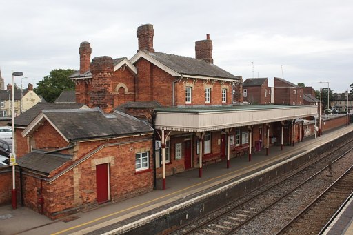
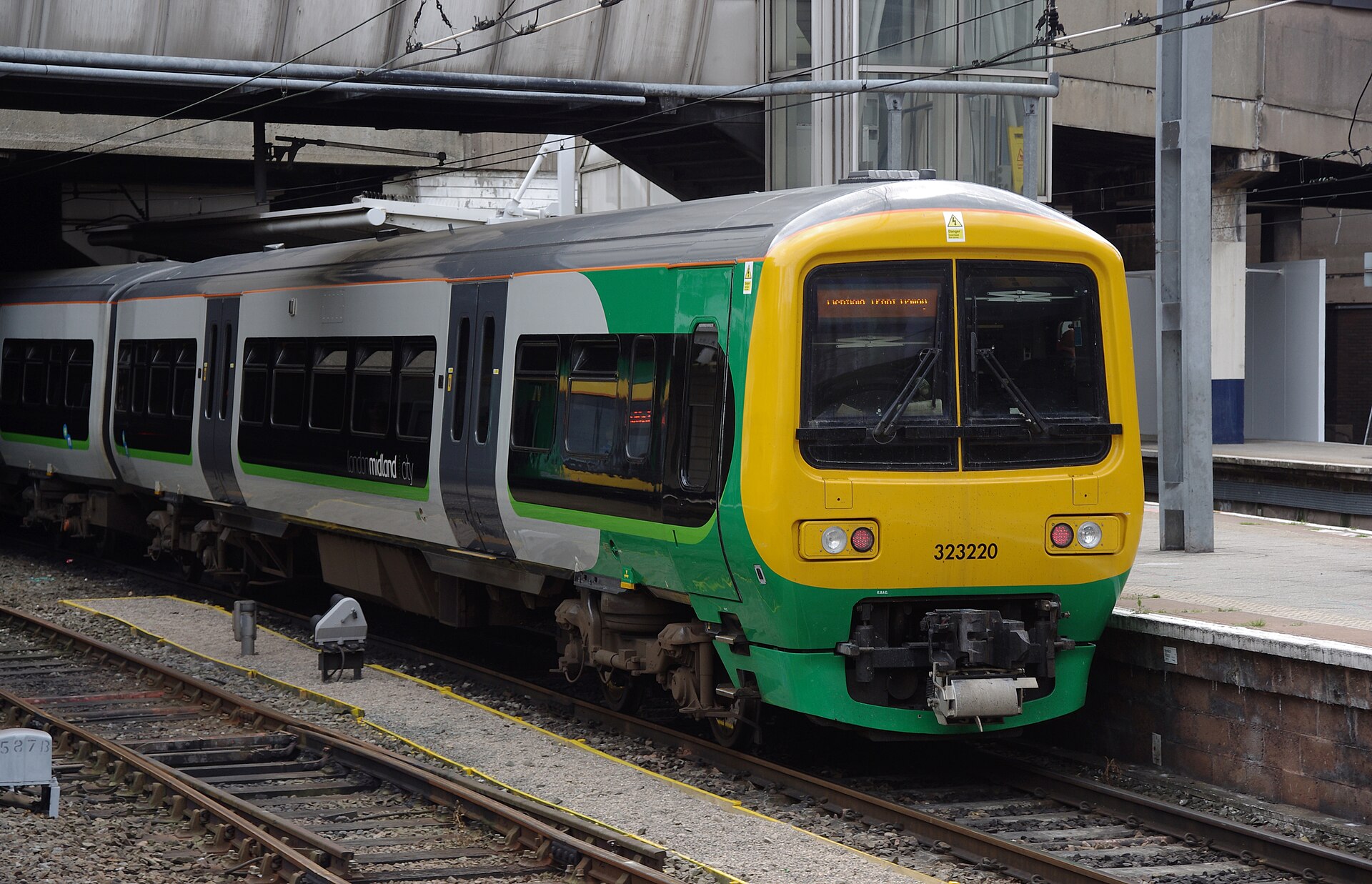
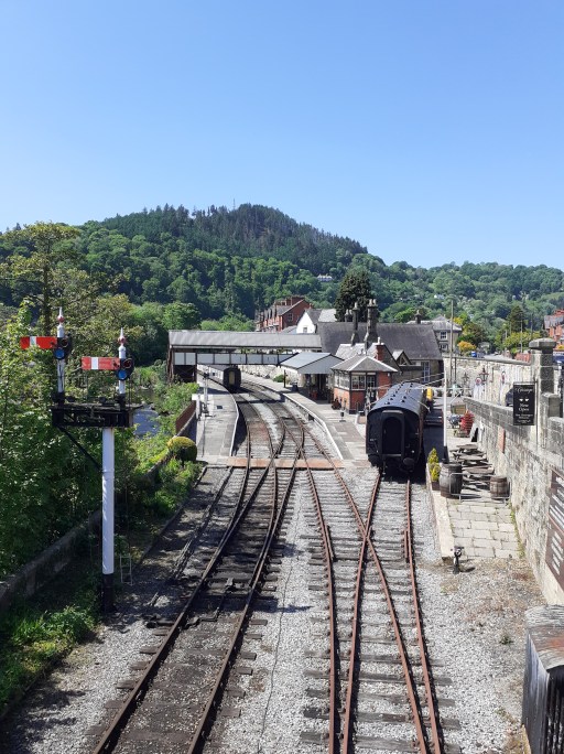
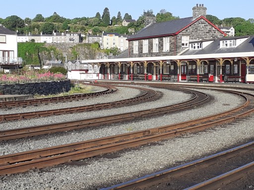
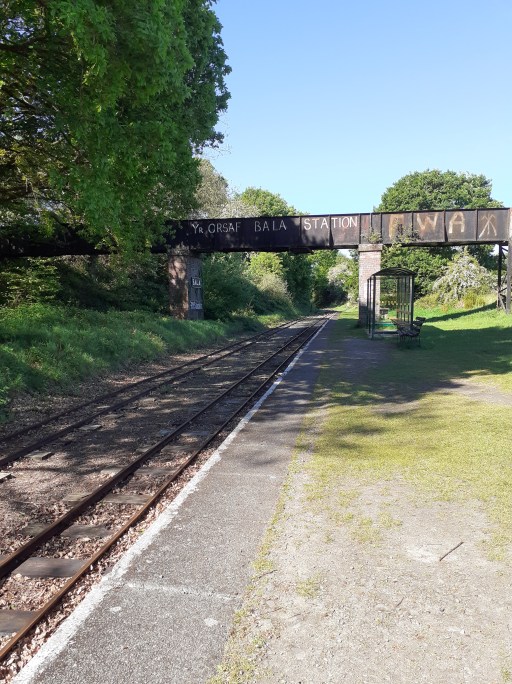
In mid-May 2025, I made a journey that I have had in mind for a number of years – a circular trip around North Wales mainly by inter-urban bus. I had a number of reasons for wanting to make this trip. Firstly it involves travel through some of the loveliest countryside anywhere in Britain. Secondly, it allowed me to indulge my obsession with looking at heritage railway stations, three of which are shown below – I will leave it to the reader to identify them. And thirdly, and for the purpose of this post most importantly, it allowed me to travel on the Traws Cymru bus network. I have watched this network develop from afar over the years, and have often thought I would like to look at it more closely.

In what follows I firstly describe the route that I took and comment on some general aspects. I then consider the vehicles that I travelled on, and then the infrastructure – bus stops and interchanges. Finally I make a number of comments on the good and bad points of the trip.

The route

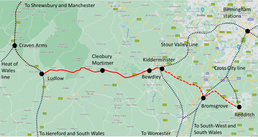
The first step of my journey was to travel from my home in Oakham in Rutland to Ruabon on the Welsh border by train. This involved changes ta Birmingham New St and Shrewsbury. There were no problems either on the way there or the way out, with all journeys running close to time. At the start of the journey there was the perennial feeling of relief when it became clear my Cross Country train was really running and had not been cancelled, that turned into a feeling of surprise when it actually arrived at Oakham on time. But, as I say, the journey worked well and I arrived at Ruabon around noon as planned.

Traws Cymru network (from the Traws Cymru web site)

The Traws Cymru inter-urban bus network in North Wales is shown in the figure above. My first bus was not however part of the Trwas Cymru network, but rather the Arriva 5 from Wrexham to Llangollen that I boarded at Ruabon. I took this rather than wait an hour and a half for the first Traws Cymru T3 bus, and it gave me time for a brief look around Llangollen and a look at the railway station. On boarding this bus I asked for a concessionary 1bws ticket (£4.70 for all day travel on buses in North Wales for English bus pass holders – excellent value). The driver looked a bit mystified but eventually gave me the correct ticket. The bus was quite full – over 50% loaded – but fairly comfortable and made up some of the time after a 10 minute late departure from Ruabon. From then on my journeys were all (bar one) on the Traws Cymru network as follows (approximate loading given in brackets).

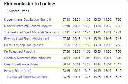
Llandudno 13.39 to Corwen 14.04 – T3 (60%)
Corwen 14.15 to Betws-y-Coed 15.03 – T10 (5%)
Betws-y-Coed 15.05 to Caernarfon 16.23 – S1 (30 to 50%)
Caernarfon 17.05 to Porthmadog 18.05 – T2 (100%+)

And the following day.

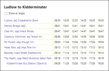
Porthmadog 8.05 to Dolgellau 9.02 – T2 (30%)
Dolgellau 9.03 to Bala 9.33 – T3 (5%)
Bala 11.33 to Ruabon 12.39 – T3 (25%)

All the journeys kept time very well, and none was more than 3 or 4 minutes late at the point where I disembarked. Throughout the trip, the drivers were helpful and friendly, which makes a hige difference to the passenger experience. The journey not on the Traws Cymru network was the Sherpa S1. I chose to change onto this, rather than continue on the T10 to Bangor and catch the T2 to Caernarfon and Porthmadog there, simply because the ride up to Pen-y-Pass at the foot of Snowdon must be one of the most spectacular and exhilarating in the country.

The vehicles

I am by no means a bus expert, but from what I could gather from various websites, I travelled on the following vehicles.

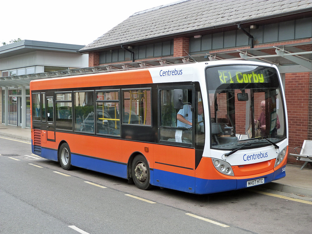
5 – ADL Enviro400 City, operated by Arriva
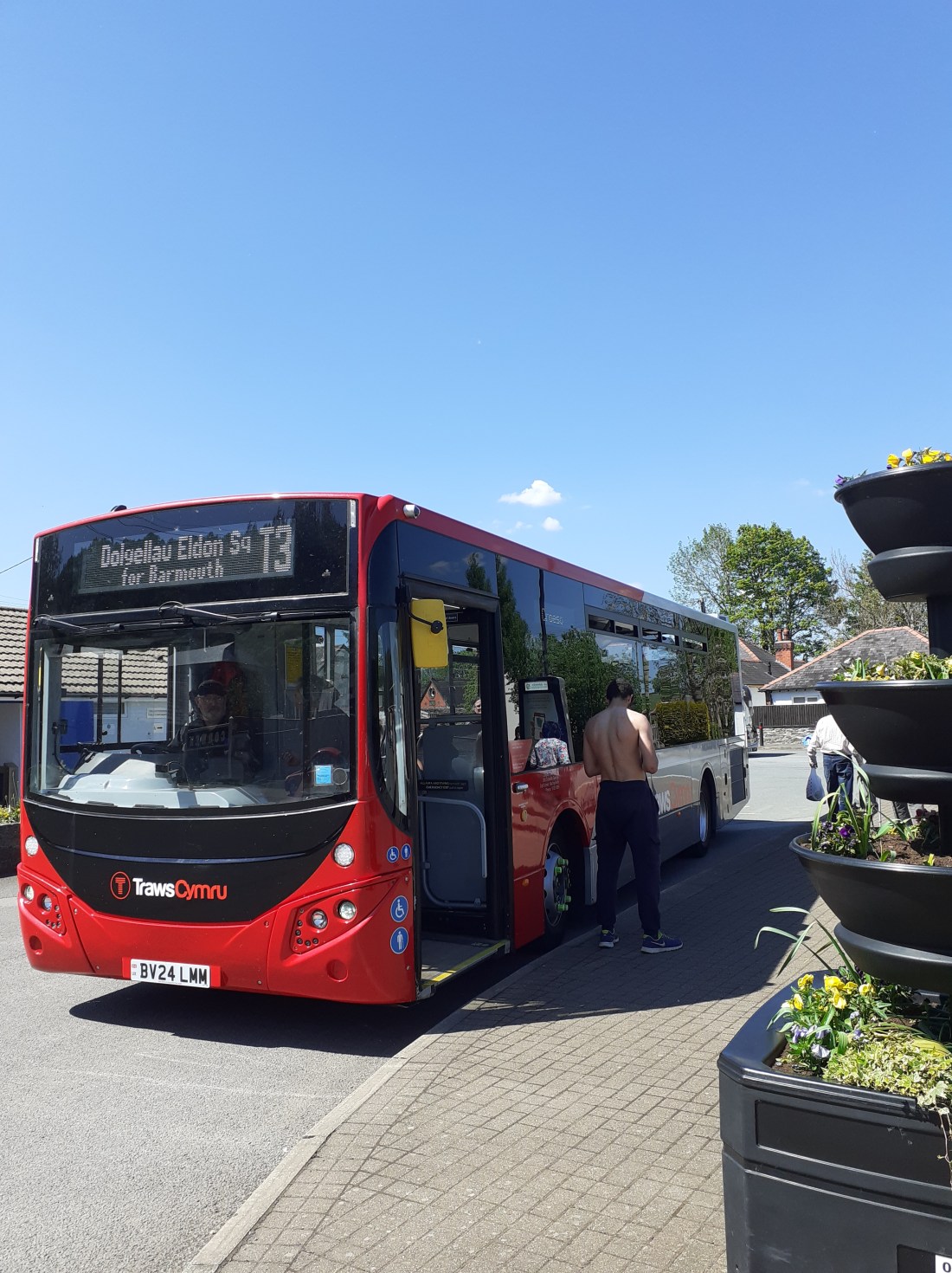
Traws Cymru T2 and T3 – Volvo B8RLE MCV Evora operated by Lloyds Coaches.
Traws Cymru T10 – ADL Enviro200 MMC operated by K and P coaches.
Sherpa S1 – ADL Enviro400 operated by Gwynfor coaches.

Photographs of all but the first of these are shown below

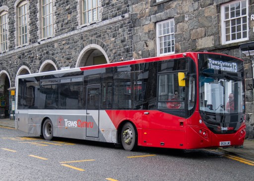
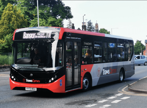
From my point of view as a passenger, the Traws Cymru and Sherpa vehicles were all basically buses – comfortable enough, with nice seats, but not of express coach standards. All vehicles had working USB charging points (something that many rail franchises don’t seem to be able to provide), and two of the Traws Cymru vehicles had WiFi, although this tended to drop out in the more rural areas. Most had screens that could potentially be passenger information screens, although they were not in use. As someone who isn’t terribly well acquainted with the area, the use of such screens to tell me which stop was coming next would have been really useful, and would have meant that I did not have to rely upon Google maps. In general though, I found the buses a pleasant and efficient way to travel, although I doubt I would have found them terribly comfortable for journeys of much more than an hour.

Bus stops and interchanges

Bus stops and interchanges are an integral part of any public transport journey, but in my experience receive far less attention and allocation of resources than they should. These feelings were reinforced on the journey described in this post

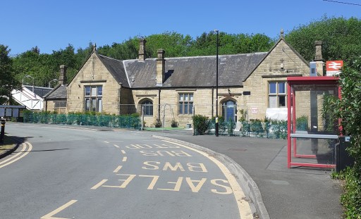
At Ruabon the Traws Cymru stop was just outside the station building. It contained basic information about timetables, but no real time information. The shelter was functional but nothing more. I actually only used this stop on my return journey – the Arriva 5 left from a stop at the end of the Station Drive. Here the same information (about northbound buses to Wrexham only) was being displayed in the shelters on either side of the road, which was confusing to say the least. If one didn’t have a basic grasp of the geography of the area, it would be easy to have got on the wrong bus.

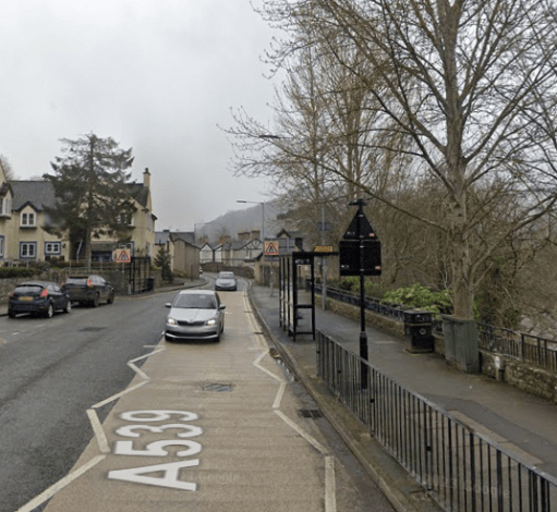
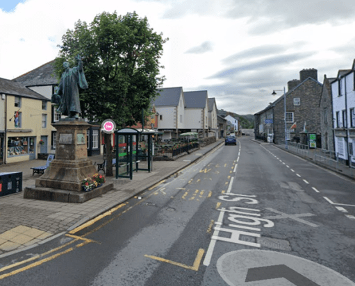
At Llangollen I got off and on the bus at the Bridge Hotel stop. This can be seen to be a roadside stop of the most basic sort. Fortunately it wasn’t raining. There was a timetable displayed, but no real time running information.

Llangollen Bridge Hotel stop (from Google Street View)

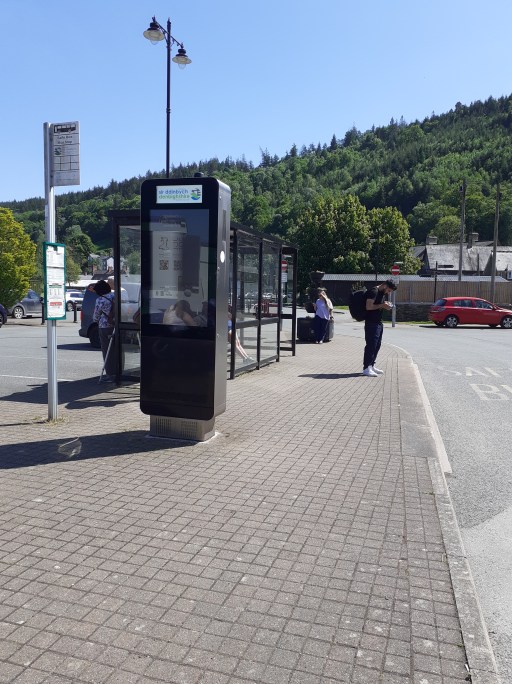
Corwen was very different. Here there are proper interchange facilities with good, real time information, a solid shelter and space to wonder in the bus stop area. I think I could make out a toilet block too, but didn’t investigate it. This is a nice facility. It would probably benefit from not being branded as “Corwen Car Park” – although it is indeed in the centre of a car park. It is much better than such a name would suggest. My only worry would be that the shelter would not be large enough for all those changing vehicles on a wet day. But this is how it should be done.

Corwen bus stop, waiting area and information panel

Corwen station on the Llangollen railway

Betws-y-Coed interchange (from Google Street View)

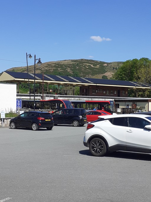
Betws-y-Coed is a strange place. It seems to be drowning in an ever expanding sea of car parks that have obliterated whatever it was that attracted folk there in the first place. The interchange is close to the station, and whilst there is shelter and some timetable information, I found the interchange, with four buses parking in an area that simply wasn’t large enough, very confusing and unsettling. Indeed I boarded the wrong bus at my first attempt. I think that there is scope for producing something like Corwen here, but it will cost I guess. Sadly the adjacent railway line, with its not-quite three hour interval service simply isn’t part of the interchange game here, which is based on a regular two hourly frequency.

Caernarfon bus station is simply a row of three of four bus stop and bays along a narrow street. However there is good passenger information and the provision of shelters is adequate. No problems here from my perspective.

Porthmadog Australia (from Google Street View)

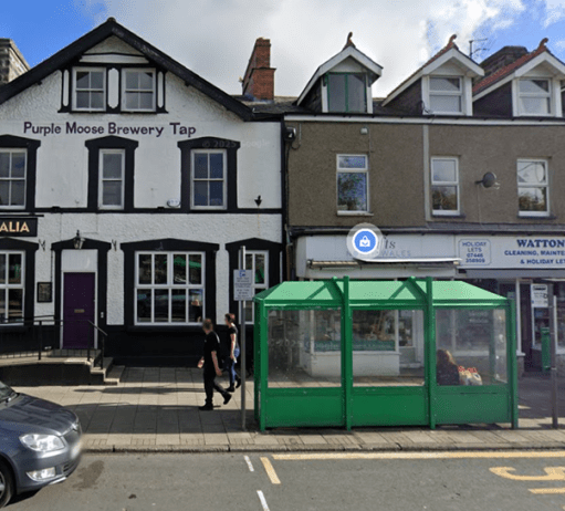
I began my second day at the bus stop outside the Australia in Porthmadog. It is simply a roadside stop. Passenger information and creature comforts are minimal. Porthmadog deserves better.

With my trip almost over, it reached its low point – Eldon Square in Dolgellau. This was perhaps the most chaotic bus interchange I have ever experienced with four buses double parked in wholly inadequate, highly trafficked space. There may have been public information systems, but such was the chaos I couldn’t find anything. The place is simply not fit for purpose. It is clear from a web search that its inadequacy is well appreciated and there have been long term discussions about how to overcome the issues. Maybe something will be sorted out in future, but of all my memories of the trip, Eldon Square is the one that remains with me. I will do my utmost to avoid ever having to use it again.

My final change of buses was at Bala – simply alighting at the stop in the centre and getting on the next bus in two hours time. again, it was a simple roadside bus stop. with only a paper timetable provided, amongst a sea of notices pasted to the stop itself. Very oddly, one of these was advertising a vacancy for a clergyman in East Sussex!

Some closing thoughts

On balance I was quite impressed by the Traws Cymru network. The regularity and timekeeping were impressive (although I suspect the latter might suffer when the traffic is busier in the high season) and the tickets were excellent value. The buses were comfortable, at least for journeys up to an hour or a little longer. It would be good if more use could be made of the on board information screens, particularly for passengers who don’t know the area well. The bus stops and interchanges were not so impressive however, with only just tolerable information provision (and hardly any in real time) and shelter provision in most places. I suspect if the weather had been wet, I would have been less impressed by the experience. The contrast between my experience at the well thought out interchange at Corwen and the chaos of Eldon Square in Dolgellau was quite stark. Something really does need to be done about the latter.

A recent news item indicates that an express North / South Wales coach service is under consideration, over the route of the current T2 to Aberystwyth and the T1 from there to Carmarthen, which would only have a relatively small number of stops in the larger towns. From my perspective this is to be welcomed, but I would urge anyone involved in implementing such a scheme not to forget the passenger infrastructure where the coach calls. If a premium service is to be provided by high quality coaches, then this must be matched by higher quality passenger facilities at its calling points, with good quality shelter and information systems – and ideally toilets and access to refreshments. Good interchange with the rail network should also be provided, with something better than a bus stop in the station carpark, Without such provision I fear any such experiment will fail.

Public Transport in Oakham from the 1960s to the present

Introduction

In this post we will consider how bus and train transport in Oakham has changed from the 1960s to the present day, for both good and bad. To do so, we will use a variety of historical resources, primarily old bus and rail timetables. We will look at four time slices – at the state of the railways in the early 1960s i.e. before the Beeching cuts; at the bus services and train service provided in the late 1960s, after Beeching but before bus deregulation; in the late 1990s after rail privatization and bus deregulation; and the current situation. The time slices chosen have in effect been determined by what information is available. However, between them they give a clear picture of how bus and train services in Oakham have developed (or perhaps degraded) over the last 50 to 60 years.

Sources and limitations

For the early 1960 rail services we use the following sources:

London Midland Region timetable for 1963 and 1965 (personal collection);
Bradshaw’s Guide 1961 (from Timetable World).

These are quite comprehensive and give a full coverage of the rail services at that time, which is of course before the Beeching Report and associated closures. The sources for the late 1960s are both taken from Timetable World:

London Midland Region timetable for 1969;
Bus timetables for the late 1960s.

Whilst the rail timetables can again be expected to be comprehensive, the bus timetables are probably less so. Finding services through Oakham requires a search of the index for bus companies operating in the area. It is possible that I have missed some potential sources of information, although I believe I have captured most of the main services. What I have almost certainly missed are any very local services operated by small operators in the Oakham district, which simply do not appear on the Timetable World web site. The bus timetables are from the years 19868 and 1969 with one exception from 1973 (for a Saturday only service). For the late 1990s we obtain information from the following sources:

Railtrack Great Britain timetable for 1999 (from Timetable World);
Great Britain Bus Timetable 1999 (personal collection).

The Great British Bus Timetable is a compilation of services from across Great Britain. It admits that it excludes local operators and services of a purely local nature, so again the bus information might not be fully comprehensive here. For the current situation we used information for bus and train times that is available on the web as follows:

Operators

In the analysis that follows, we will identify bus and train operators by a two letter code.

BL – Blands of Cottesmore – a local bus company based in a village to the east of Oakham.
BA – Bartons or Barton Tobin Hood – a large regional bus company based around Nottingham, but with a garage in Stamford.
BR – British Rail – the National pre-privatisation rail operator.
CB – CentreBus – an East Midlands regional operator.
CC – Cross Country Trains – the current franchise operator of trains through Oakham, with a wide nationwide network.
CT – Central Trains – a previous operator of trains through Oakham, based in Birmingham with a wide regional network across the Midlands.
EM – East Midlands Railway – the mainline train operator serving the East Midlands cities, that runs occasional services through Oakham (and is, bizarrely, the firm responsible for running the station).
KI – Kinchbus – a small Loughborough based bus company
LR – Lincolnshire Road Car – a large regional company in the 1960s, primarily based, as might be expected, in Lincolnshire.
MR – Midland Red Leicester – the regional operator of the very large Midland Red network that operated buses across the wider Midlands area.
RC – Rutland County Council – which currently operates a small number of services for which no franchise partner could be found.
UC – United Counties Omnibus Company – a large regional company primarily based in the Northampton area.

Analysis

In what follows we consider the public transport services through time in four categories:

Local interurban services to Stamford, Melton Mowbray and Uppingham;
Regional services to Peterborough, Leicester, Nottingham, Grantham and Corby;
Long distance services to Birmingham, Cambridge and London;
Miscellaneous services for which information is incomplete – very local services, long distance coaches etc.

For the first three categories we present the data in tabular form in a consistent format, and then discuss how these have evolved over time. Discussion of the latter category is inevitably rather more diffuse due to the lack of much historical information.

Local interurban services

Tables 1 to 3 show, in standard form, the bus and train services between Oakham and Stamford, Melton Mowbray and Uppingham. Journey times and number of journeys / day are shown. Clearly there are both train and bus options to Stamford and Melton Mowbray, but only bus options to Uppingham. The bus journeys in 1969 and 1999 were provided by major bus operators for which Oakham was at the edge of their operating area – United Counties in Northampton, Lincolnshire road Car, Bartons in Nottingham, Kinchbus in Loughborough. Currently they are provided by more local operators – primarily Blands, but with Rutland County Council running the current Oakham to Stamford service. The bus journey times and service frequencies have remained similar over the period (although note that the former can vary significantly depending on what villages are served on the way between urban centres. The loss of Sunday services is obvious from the data in the tables. What is not so obvious is the fact that evening services on all the bus routes have been significantly cut over the study period.

By contracts the train services have seen major improvement. The Leicester to Peterborough shuttles stopped at all the village stations before Beeching and the journey times between Oakham and Melton Mowbray and Stamford were of the order of 20 minutes. By 1969 these stations had closed and the journey times significantly reduced. This reduction has continued up to the present with faster stock being introduced on the line and, most significantly, the number of journeys has increased by a factor of two with the introduction of hourly through Birmingham to Cambridge / Stansted Airport services. These improvements have however resulted in a significant loss of connectivity to the villages where stations were closed in the 1960s.

Table 1. Oakham to Stamford

Uppingham to Stamford via Ridlington, Wing, Oakham (Railway Station Crossing), Exton, Whitwell, Empingham and Great Casterton. UC also operated service 280 with one return journey on Fridays only from Oakham to Stamford vis Edith Weston.
Oakham to Stamford via Whitwell, Empingham and Great Casterton.
Oakham to Stamford via Whitwell, Empingham and Great Casterton. BL185 has one service from Monday to Friday and four on Saturday. RCR9 has five services Monday to Friday.
Leicester to Peterborough East via Syston, Frisby, Melton Mowbray, Saxby, Ashwell, Oakham, Manton for Uppingham, Luffenham, Ketton and Collyweston, Stamford, Helpston and (for some journeys) Peterborough North.
Leicester to Peterborough via Melton Mowbray, Oakham and Stamford
Birmingham to Cambridge / Stansted Airport via Leicester, Melton Mowbray, Stamford and Peterborough.
Birmingham to Cambridge / Stansted Airport via Leicester, Melton Mowbray, Stamford and Peterborough. Also, two early morning / late evening EM services from Nottingham to Norwich calling at Loughborough, Melton Mowbray, Stamford and Peterborough (not included in table).

Table 2. Oakham to Melton Mowbray

Melton Mowbray to Oakham (Station Approach) via Whissendine, Ashwell and Langham. Also, four journeys / day Oakham to Langham only.
KIRF (Rutland Flyer) Corby to Melton Mowbray via Uppingham, Oakham and Cottesmore; BA2 Uppingham to Nottingham via Oakham, Langham, Whissendine and Melton Mowbray.
BLR1 Corby to Melton Mowbray via Uppingham, Oakham, Langham and Whissendine; CBR2 is Oakham to Melton Mowbray via Exton, Cottesmore and Whymondham. Also, one BLR4 service per day Melton Mowbray to Peterborough via Oakham and Uppingham (not shown in table).
Leicester to Peterborough East via Syston, Frisby, Melton Mowbray, Saxby, Ashwell, Oakham, Manton for Uppingham, Luffenham, Ketton and Collyweston, Stamford, Helpston and (for some journeys) Peterborough North.
Leicester to Peterborough via Melton Mowbray, Oakham and Stamford.
Birmingham to Cambridge / Stansted Airport via Leicester, Melton Mowbray, Stamford and Peterborough.
Birmingham to Cambridge / Stansted Airport via Leicester, Melton Mowbray, Stamford and Peterborough. Also, two early morning / late evening EMT services from Nottingham to Norwich calling at Loughborough, Melton Mowbray, Stamford and Peterborough (not included in table).

Table 3. Oakham to Uppingham

Uppingham to Stamford via Ridlington, Wing, Oakham (Railway Station Crossing), Exton, Whitwell, Empingham and Great Casterton.
KIRF (Rutland Flyer) Corby to Melton Mowbray via Uppingham, Oakham and Cottesmore; BA2 Uppingham to Nottingham via Oakham, Langham, Whissendine and Melton Mowbray.
Corby to Melton Mowbray via Uppingham, Oakham, Langham and Whissendine

Regional interurban services

In this section we consider the evolution of services from Oakham to the major surrounding conurbations of Peterborough, Leicester, Nottingham, Grantham and Corby (Tables 4 to 8). With regard to Peterborough and Leicester, the same remarks can be made as in the last section in terms of the rail services, with steadily decreasing journey times and a major improvement in service frequency. For both towns there have only ever been occasional and sporadic bus links, addressing specific leisure, employment or educational needs, with long journey times. Direct services to Grantham were an early casualty of service rationalization and were not provided after the early 1970s.

In the early 1960s train services were provided from Nottingham to Melton Mowbray, Oakham, Corby, Kettering and beyond. Services on this line were a major casualty of the Beeching closures and there are now only very limited rail services to both Nottingham and Corby. Whilst there was quite a good bus service from Oakham to Nottingham in 1999, operated by Barton, this did not last and there are now no direct bus services to that city. There are, however, regular services to Corby that run through Oakham to Melton Mowbray. In 1999 these were provided by Kinchbus and marketed as the Rutland Flyer. Now the service is operated by Blands. Journey times are of the order of 40 to 50 minutes.

Table 4. Oakham to Peterborough

Melton Mowbray to Peterborough via Langham, Oakham, Uppingham and South Luffernaham.
Leicester to Peterborough East via Syston, Frisby, Melton Mowbray, Saxby, Ashwell, Oakham, Manton for Uppingham, Luffenham, Ketton and Collyweston, Stamford, Helpston and (for some journeys) Peterborough North
Leicester to Peterborough via Melton Mowbray, Oakham and Stamford
Birmingham to Cambridge / Stansted Airport via Leicester, Melton Mowbray, Stamford and Peterborough.
Birmingham to Cambridge / Stansted Airport via Leicester, Melton Mowbray, Stamford and Peterborough. Also, two early morning / late evening trains from Nottingham to Norwich calling at Loughborough, Melton Mowbray, Stamford and Peterborough (not included in table).

Table 5. Oakham to Leicester

Saturdays only. Oakham (Station Road) to Leicester via Braunston, Knossington, Cold Overton and Melton Mowbray.
Leicester to Peterborough East via Syston, Frisby, Melton Mowbray, Saxby, Ashwell, Oakham, Manton for Uppingham, Luffenham, Ketton and Collyweston, Stamford, Helpston and (for some journeys) Peterborough North.
Leicester to Peterborough via Melton Mowbray, Oakham and Stamford
Birmingham to Cambridge / Stansted Airport via Leicester, Melton Mowbray, Stamford and Peterborough.
Birmingham to Cambridge / Stansted Airport via Leicester, Melton Mowbray, Stamford and Peterborough. Also two early morning / late evening trains from Nottingham to Norwich calling at Loughborough, Melton Mowbray, Stamford and Peterborough (not included in table).

Table 6. Oakham to Grantham

Oakham (Railway Station) to Grantham, calling at Cottesmore, Greetham, Market Overton and Thistleton. Also 3 journeys from Oakham to Cottesmore only.

Table 7. Oakham to Nottingham

Nottingham to Uppingham via Melton Mowbray, Whissendine, Langham and Oakham.
Nottingham to Kettering, via Old Dalby, Melton Mowbray, Oakham, Manton for Uppingham, Gretton, Corby and Kettering, Two or three of these were from Nottingham (and beyond) to London St Pancras.
Nottingham to Norwich calling at (Leicester), Loughborough, Melton Mowbray, Oakham, Stamford and Peterborough (early morning and late evening only)

Table 8. Oakham to Corby

Corby to Melton Mowbray via Uppingham, Oakham and Cottesmore.
Corby to Melton Mowbray via Uppingham and Oakham
Nottingham to Kettering, via Old Dalby, Melton Mowbray, Oakham, Manton for Uppingham, Gretton, Corby and Kettering. Two or three of these were from Nottingham (and beyond) to London St Pancras.
Melton Mowbray to London St Pancras calling at Oakham and Kettering.

Long distance services

The three long-distance services we consider are Oakham to Birmingham, Cambridge and London (Tables 9 to 11). All of these are rail based. The first two reflect the changes described above to the Leicester to Peterborough services with a significantly increased number of services and steadily reducing journey times. The London situation is very different. When services ran from Nottingham to London via Oakham in the early 1960s, there were four trains to and from London each day. After Beeching these were withdrawn completely and it is only in recent years that one journey, from Melton Mowbray to London has been reinstated. Thus whilst there has been considerable improvement in east / west connectivity, north / south connectivity has been reduced to a nominal level.

Table 9. Oakham to Birmingham

Birmingham to Cambridge / Norwich via Leicester, Melton Mowbray, Stamford and Peterborough.
Birmingham to Cambridge / Stansted Airport via Leicester, Melton Mowbray, Stamford and Peterborough.
Birmingham to Cambridge / Stansted Airport via Leicester, Melton Mowbray, Stamford and Peterborough

Table 10. Oakham to Cambridge

Birmingham to Cambridge via Leicester, Melton Mowbray, Stamford and Peterborough.
Birmingham to Cambridge / Stansted Airport via Leicester, Melton Mowbray, Stamford and Peterborough. Birmingham to Cambridge / Stansted Airport via Leicester, Melton Mowbray, Stamford and Peterborough

Table 11. Oakham to London

Nottingham to Kettering, via Old Dalby, Melton Mowbray, Oakham, Manton for Uppingham, Gretton, Corby and Kettering. Two or three of these were from Nottingham (and beyond) to London St Pancras.
Melton Mowbray to London St Pancras via Oakham and Kettering

Other services

When looking at the information available from the sources listed above, it is clear that there are two broad categories of bus service that are not fully represented – very local services in and around Oakham and the nearby villages; and long-distance coach services. With regard to the former, it is known that local companies such as Blands provided specific services to places of work and education and indeed that still continues in the latest timetable. These are usually one or two journeys a day with no wider public transport relevance. Als Rutland County Council operate a minibus Rutland Hopper service around the town to out-of-town stores and local villages.

It is also clear that some long distance coaches operated through Oakham, but these are not easy to find, usually occurring in specific operators timetables. For example, in 1968 Barton operated a long-distance coach service between Corby and Glasgow (presumably for steel worker s to visit families), with daytime trips on Sunday, Monday and Wednesday, and overnight trips on Friday and Saturday, that picked up and dropped off at the Crown Hotel. Similarly in 1969 Trent Motor Traction, based in Derbyshire and Nottinghamshire ran weekend services from Derby and Nottingham to Southend on Sea, Cambridge and Clacton that ran through Oakham, picking up and setting down at the Market Place. There were no doubt other similar occasional services.

Conclusions

So what can one conclude from the data presented above? Firstly with regard to rail services, it is clear that there have been major improvements in connectivity to the east and the west, with reducing journey times and increased frequencies. That being said, current reliability and punctuality is poor and requires improvement. Services to the north and south have however seen major degradation and are now only represented by one journey a day to London. With regard to bus services, in some sense these have seen little change, with journey times and frequencies on most routes remaining broadly constant, at least on weekdays. That being said, there have been some losses – to Grantham and Nottingham in particular, Sunday services are non-existent and evening services have been severely cut back, Perhaps more importantly the service times and frequencies that were acceptable in the 1960s now simply represent a very basic service that is not attractive to most car-owning travelers.

An election manifesto for Transport

Introduction

As the journalist Christian Wolmar has discussed in a recent article, the UK does not have any sort of agreed National Transport Policy that could be used as a rational way of developing transport infrastructure in a politically non-partisan way. Such a policy will certainly not emerge from the current government, and there is little to suppose that any future government will give priority to developing such a plan. Without it, transport policy is vulnerable to ill thought-out ad hoc initiatives and, as at present, in ad hoc cutbacks. In this post I will suggest a pragmatic way forward on this.

What I propose is based on the assumption that the next Government will be formed by the Labour Party, either as a majority party or with some sort of agreement with the Liberal Democrats. This is certainly what would be suggested by the opinion polls where at the time of writing Labour have a 22% lead over the conservatives. The Labour party has proposed five “missions” that will direct their approach to the 2024 elections and any subsequent government. None of these missions mentions transport at all, but there are transport issues embedded in each one of them. In what follows, I set out these missions, the transport issues that arise from them, potential policy objectives, and potential policy proposals. I then bring these proposals together to form a list of Transport policies that could be used, no doubt in a modified format, both for the next election and in any subsequent government.

Readers should not assume from this that I am a Labour Party supporter. I have never been a member of a political party, and never intend to be. Politically I am a centrist, but with somewhat radical environmental views, formed partly by my professional work as a Professor of Environmental Fluid Mechanics at the University of Birmingham (now retired). The proposals below are simply pragmatic – a possible way of influencing the next government to do something sensible in transport terms.

The Labour Part Missions

Mission 1

Secure the highest sustained growth in the G7, with good jobs and productivity growth in every part of the country making everyone, not just a few, better off.

Transport issues

Transport congestion on road and rail, for both people and products, leading to reduced productivity.
Poor workforce mobility, leading to inflexibility in employment locations.
DfT methodology for assessing CBR of transport infrastructure does not take proper account of induced flows on highways – i.e. new roads encourage traffic growth and can increase congestion.

Transport policy objectives

Revise DfT methodology for assessment of congestion reduction of new roads to include induced flow effects.
Infrastructure interventions to reduce road and rail congestion.
Encouragement of modal shift from road to rail, for both people and products.

Transport policy proposals

Revision of DfT methodology for assessing congestion reduction of new road schemes to include proper consideration of induced flow.
Small number of specific congestion-reducing road schemes (consistent with Mission 2).
Speed up development of rail enhancements and new build (HS2, EWR and NPR).

Mission 2

Make Britain a clean energy superpower to create jobs, cut bills and boost energy security with zero-carbon electricity by 2030, accelerating to net zero.

Transport issues

DfT methodology for assessment of contribution new transport schemes to carbon production and climate change has been shown to be flawed, particularly in relation to new roads.
UK Carbon based transport emissions levelling off or increasing.
Transport is now major carbon producing sector of economy.

Transport policy objectives

Reassessment of DfT methodology for assessing environmental impact and carbon production of new transport schemes.
Development and roll out low carbon technologies (electric and hydrogen vehicles, electric trains) including electric car recharging infrastructure.
Encouragement to use low carbon modes of transport and active travel modes.

Transport policy proposals

Revision of DfT methodology for assessing environmental impact of new road schemes to be revised.
Investment in electric and hydrogen vehicle research and production
Development of electric vehicle recharging infrastructure.
Electrification programme for railways
Fiscal incentives to encourage low carbon mode use.

Mission 3

Build an NHS fit for the future by reforming health and care services to speed up treatment, harnessing life sciences and technology to reduce preventable illness, and cutting health inequalities.

Transport issues

Poor air quality in urban areas mainly due to transport, leading to vulnerability to respiratory illness and, possibly, increased dementia risk.
Contribution to high levels of obesity due to short journeys being made by car.
Poor access to health facilities for those without cars (20% of households)

Transport policy objectives

Improve urban air quality through encouraging low emission vehicles.
Improve air quality through traffic reduction and modal shift to public transport.
Encourage active travel (cycling and walking).
Improve public transport (primarily bus) links to health care facilities,

Transport policy proposals

Fiscal incentives for ULEZs and LTNs.
Support for public transport
Fiscal incentives to local authorities to provide active travel infrastructure.

Mission 4

Make Britain’s streets safe by reforming the police and justice system, to prevent crime, tackle violence against women, and stop criminals getting away without punishment.

Transport issues

Safety issues due to high road speeds in urban areas.
Safety issues due to pavement parking.

Transport policy objectives

Make urban streets safe for pedestrians and cyclists.

Transport policy proposals

Fiscal incentives for LTNs.
Lower and enforce urban speed limits.
Enforce pavement parking laws.

Mission 5

Break down the barriers to opportunity at every stage, for every child, by reforming the childcare and education systems, raising standards everywhere, and preparing young people for work and life.

Transport issues

Poor access to childcare and education for those without cars (20% of households)

Transport policy objectives

Improve access to childcare and education for those without cars.

Transport policy proposals

Support for public transport
Fiscal incentives to local authorities to provide active travel infrastructure.

The policies

From the consideration of the individual missions, the following specific transport policies can be developed.

Policy 1

Revision of DfT methodologies for assessing new transport schemes to take proper account on induced flow and environmental effects. (Missions 1 and 2)

Policy 2

Invest in new transport infrastructure with a small number of congestion-relieving road schemes, electric car charging facilities, and major investment to rail infrastructure, including staged development of HS2, NPR and EWR) and a rolling programme of electrification. (Missions 1 and 2)

Policy 3

Support for public transport (trains and buses) for increasing employment opportunities and providing access to healthcare and education. (Missions 1, 3 and 5)

Policy 4

Reduction of urban speed limits and enforcement of pavement parking laws. (Mission 4)

Policy 5

Fiscal incentives and support to local authorities to encourage low carbon vehicles and modal transfer to low carbon modes; for the development of ULEZs and LTNs, and provision of active travel infrastructure. (Missions 2, 3 and 5)

Commentary

Policy 1 is not going to set any electoral debate alight, but it is quite crucial. In the past the DfT has used flawed policies to assess road building schemes against other transport schemes, knowing that they were flawed. This needs to change. Indeed, I would regard the DfT as no longer fit for purpose in many ways (as an example, its current handling of the railway network, the ongoing industrial action and major cutbacks to active travel budgets can be cited) and there is an argument for a complete re-organisation here to establish a wide ranging Department for Infrastructure that brings together transport, the utilities and construction. This would allow proper consideration to be given to the transport effects of new housing build (often built without public transport provision) and conversely the effect of a move to electric vehicles on the development of the electricity grid.

Policy 2 is wide ranging and expensive, and any specific proposals would need to be carefully phased in terms of expenditure. The basic point however is that high quality transport infrastructure for people and products is a fundamental requirement for a productive economy, the more so as the switch to the “green economy” proceeds.

Policy 3 is important for many, and in particular those on low incomes. The provision of a high-quality public transport network (particularly buses) that is comprehensive in its coverage would make access to employment, healthcare and education very much easier for many people.

Policy 4 is essentially aimed at public safety. It would no doubt be categorised as a “war on motorists” by sections of the press, but this is a battle that needs to be fought for the public good.

Policy 5 is another proposal that might be electorally contentious as (weirdly to my mind) LTNs, ULEZs and active travel have become very politicised. Fiscal incentives could be a way forward here, as proposed in the more detailed description of Mission 2 recently released by the Labour Party. This might include the possibility of both support for the initiatives and a wider reduction in rates for those Local Authorities that develop such schemes. This would be basically a bribe, and would need to be carefully costed and targeted, but could help in the establishment of such schemes. In terms of encouragement to use low carbon modes, a study should be initiated to look at how road pricing, aviation fuel duty and rail fares could be used to encourage the necessary modal shift.

The 292 bus route from Kidderminster to Ludlow – an important transport link?

292 at Kidderminster Bus Station in 2010

I have recently been on a short break to Cleobury Mortimer in Shropshire, travelling there by train and bus from where I live in Lichfield. The train journeys, from Lichfield to Birmingham and Birmingham to Kidderminster went very smoothly and were quite a pleasant experience. There were a number of route permutations, but we chose to walk between Birmingham New Street and Birmingham Moor Street, both on the way there and back. The bus leg from Kidderminster, on the Diamon bus 292 was rather less easy. The bus didn’t stop at Kidderminster railway station, with the nearest advertised stops (on Google and various websites) being 400m away in Oxford St. Arriving there however, we found this was not the case, with no mention of the 292 on the timetables at the stop, so we walked on to the bus station, another 400 yards away. There we eventually did get the bus, which was running over half an hour late. The journey itself was fine, and as we were in no hurry, the delay was of no particular concern to us.

Over the days that followed, I kept track of the buses on the 292 route between Kidderminster, Bewdley, Cleobury Mortimer and Ludlow, and it soon became clear that the lateness was endemic. The journey was timetabled for 50 to 55 minutes, with a two-hour frequency, with one bus shuttling backwards and forwards – see the timetable below – from https://bustimes.org/services/292-kidderminster-ludlow . This timing was simply too tight to ensure punctual running throughout the day. Whilst some of the delays came from congestion in the towns at either end of the route as might be expected, the most critical delays were due to parked cars on the A4117 between Bewdley and Ludlow requiring single file traffic through the towns and villages along the road. Such delays could of course be quite easily eliminated, given the political will.

Current 292 Timetable

Now service 292, currently operated by Diamond buses, is actually the truncated remains of a much longer Midland Red service with the same number, that ran from Birmingham to Kidderminster, Ludlow and Hereford. A time table for this service is shown below from 1991 for the Birmingham – Hereford direction – from http://midlandred.net/service/timetable/display.php?routeID=1007. The service was withdrawn, apart from the Kidderminster to Ludlow leg, in the early years of the current century. It can be seen at that time there was an hourly service between these two towns, rather than the current two hourly service. This represents a considerable degradation in service provision.

292 Timetable 1991

But the transport context has changed in many ways over the last few decades. The role of the long-distance bus has been largely taken over by trains, with a much greater frequency than 30 years ago. On the original 292 route there are now 4 trains an hour to Kidderminster from Stratford upon Avon through Birmingham, either terminating there or continuing to Worcester, and two from Worcester to Birmingham; at Ludlow there are two trains per hour in each direction between Manchester, Shrewsbury, Hereford and various destinations in south Wales. So in this sense, the truncation of the service was sensible and appropriate. It now serves a purely local market for those who live on its route. But I would argue, in any sane country that takes seriously the need to reduce carbon emissions and the need for modal change (i.e. not the one in which I reside), the Kidderminster to Ludlow route would be of some strategic importance. With improvements in frequency and connections with rail at Kidderminster and Ludlow, it would offer a route from the West Midlands conurbation, via the Stour Valley line, into south Shropshire and the Marches, with major tourist potential. Further, if the route were combined with the hourly 52 from Kidderminster to Bromsgrove (and ultimately Redditch), it would offer connections from the south west at Bromsgrove into the same area, and also from the Cross City line that serves the north of Birmingham and the city centre. The 52 actually runs past both Bromsgrove and Kidderminster stations. Continuation of the service north of Ludlow to Craven Arms (in parallel with the railway) would offer connections to the Heart of Wales line, whose tourist potential has not been fully developed, and perhaps further to Welshpool for connections to the Cambrian line. All these possible connections are shown in the figure below.

But life is of course not that simple. For such a service to be a success other changes would be necessary. Firstly, efforts would be required to split the local markets in Ludlow and Kidderminster from the longer-distance markets to make overall journey times on through services as short as possible. There is no reason why this should not be possible but would require extra resources in terms of service provision to meet the requirements of the very local market. This mix of markets has been a major reason for the demise of long distance inter-urban buses in the past – perhaps most recently in the truncation of the Oxford to Cambridge X5 at Bedford, because the local market between Bedford and Cambridge resulted in significantly increased journey times. Secondly, attention would need to be paid to the interchange points at either end of the route. For example, the bus stops of the Bromssgrove to Kidderminster route at Kidderminster Railway Station are on narrow pavements on a road bridge over the railway line – a very uninviting and inconvenient place for mode transfer. Attention would also o fcourse need to be paid to timetabling to ensure suitable connection times.

The other issue is of course more structural in that there is no overall transport policy in the UK that would facilitate such developments – see the recent blog by Christian Wolmar on this. And this lack of an overall policy means that resources cannot be channeled to such schemes, despite the fact that their benefits would be significant in terms of carbon emission reductions and stimulating local economies. It has always been thus as far as I can remember. I still want to believe that a competent government will one day realise that this is the road to take. But perhaps I am here opening myself up to a charge of naivety.

Yet more on cross winds effects on trains

Train blown over by high winds in Switzerland in March 2023

This post and its attachments continues a sporadic (and what some might call obsessional) series on the effects of cross winds on trains. It gives links to a downloadable report and a downloadable spreadsheet.

The report (below), which follows on from two papers I wrote in 2010 and 2013, presents a detailed analysis of the effects of unsteady crosswinds on trains using a simple train dynamic system methodology. This begins with the specification of unsteady wind characteristics that are then used to calculate unsteady aerodynamic forces. These are then used as input to the dynamic model to calculate lateral, vertical and rotational displacements and unsteady track forces. Three specific effects are then considered – wheel unloading criteria, track force criteria and vehicle displacement criteria, and a rigorous statistical methodology used to specify values of these under specific unsteady crosswind conditions. A simple methodology for developing wheel unloading cross wind characteristics (CWCs) is then set out and calibrated using the dynamic model. This calibration indicates that the simple model is more than adequate to determine wheel unloadings in design, and that the more complex aspects of the suspension, track roughness of spatial non-correlation of the aerodynamic loads have little effect on the calculated CWCs. Finally possible extensions to the modelling methodology are outlined – in terms of investigating a range of effects on wheel unloading dynamics, the extension of the method to investigate track forces, roof displacements and pantograph / OHL displacements in cross winds.

a-detailed-study-of-crosswind-effects-on-train-systems Download

The spreadsheet gives a simple and straightforward way of calculating the CWCs using the methodology described in the report. It is made available on the basis that the coding has not been verified in any rigorous fashion, and that the user takes full responsibility for the output. That warning being given, I hope some will find it of interest. There are two worksheets. For both the user-defined parameters are highlighted in yellow. The first calculates the CWC from a user-specified value of the characteristic velocity The second calculates the value of characteristic velocity from the vehicle geometric, mass and aerodynamic parameters as in section 11 of the above report. It uses the same values for these parameters as used in the report, but these can be changed as required.

cwc-calculator Download

Cross Wind Characteristics – a mathematical curiosity

Readers of this blog will know that one of the subjects that I have worked on over the last 40+ years has been the effect of cross winds on trains. By this time, one would have thought that I should have plumbed the depths of the topic, but it still has the ability to surprise. In this short (and very nerdy) post I want to describe a mathematical curiosity associated with this subject that I have recently become aware of.

Box 1, CWC Calculation methodology

In the book “Train Aerodynamics – fundamentals and applications” I set out a simple methodology for calculating Cross Wind Characteristics (CWCa) – essentially plots of overturing wind speed against train speed. This is based on a simple three mass model and the equations are set out in Box 1 above – equation (A) for the low yaw angle range, and equation (B) for the high yaw angle range. I won’t describe this in further detail here – the book only costs £132 on Amazon, so any interested readers can find a fuller description there and provide some minimal royalties to myself and the other authors.

Recently I have had occasion, as part of a consultancy project, to develop simple spreadsheet to enable CWCs to be calculated for a range of different types of rail vehicle. The method I chose was to solve equation (A) for low yaw angles below the critical yaw angle and equation (B) for high yaw angles above the critical angle, using the Newton Raphson iterative method. These equations give an explicit solution for the overturning wind speed at a train speed of zero. The value of train speed is then increased in small increments up to the vehicle maximum operating speed, with the first estimate in the iteration at any one wind speed being the converged value of wind speed from the previous calculation with a slightly lower train speed. Convergence is usually very rapid, usually just one or two iterations.

Figure 1 Calculated CWCs for n₁=1.5, n₂=0 for wind directions up to 90 degrees

Figure 2 Calculated CWCs for for n₁=1.5, n₂=0 for wind directions above 90 degrees

Figure 3 Calculated CWCs for for n₁=1.5, n₂=-0.5 for wind directions above 120 degrees

The methodology in general worked well, and some of the results for different wind directions relative to the train direction of travel are shown in Figures 1 and 2 (for lee rail rolling moment coefficients at 30 and 90 degrees of 2.2 and 3.5 respectively and parameters n₁ and n₂ of 1.5 and 0.0, i.e. a steadily increasing rolling moment coefficient up to the critical yaw angle, and a constant value above that angle). The two yaw angle ranges can be clearly seen, with the lower yaw angle range at the higher train speeds, and the higher yaw angle range at the lower train speeds. For the train aerodynamic characteristics shown here, the calculations are very stable up to a wind direction of 120 degrees. However, if the calculation is carried out for higher wind directions, then something odd happens and the iteration becomes unstable as can be seen for the 135 and 150 degree cases in figure 2. This effect is even more severe for different rolling moment characteristics. Figure 3 shows the CWCs for the same rolling moment coefficients and value of n₁, but with a value of n₂=-0.5 and thus with a peak at the critical yaw angle, which is typical of high-speed trains. Here we can see major instabilities for wind directions above 120 degrees. I was very puzzled as to why this was the case. Whilst in practical terms this is of no significance, as the overturning wind speeds for such wind directions are high and not close to the minimum critical value at any one vehicle speed, but nonetheless it would still be good to understand what was going on.

After playing around with the equations for a while, I found the best way to understand this was to regard equations (A) and (B) as quadratic equations in train speed and solve for train speed for a range of values of overturning wind speed. This is the wrong way round of course, as the vehicle speed is really the independent variable that can be specified, and the wind speed is the dependent variable that needs to be calculated but solving the equations in this way proved to be illustrative.

As the equations are quadratics, there are two solutions for train speed for each value of wind speed for each equation, and regions of the vehicle speed / wind speed plane where no solutions exist. There are thus four distinct solutions to the equations, two for the low yaw angle range and two for the high yaw angle range. These are shown for a range of different wind directions in Figure 4 for the same case as in figures 1 and 2. Here the solutions are shown for both positive and negative train speeds. The critical yaw angle condition is indicated by the short-dotted lines – between the lines the high yaw angle curves will form the CWC and outside them the CWC will be formed from the low yaw angle curves. The calculated CWCs (in the positive velocity quadrant) are shown by the long-dotted line.

a) Wind direction = 30 degrees

b) Wind direction = 60 degrees

c) Wind direction = 90 degrees

d) Wind direction = 120 degrees

e) Wind direction = 150 degrees

Figure 4 Complete solutions of equations A and B for for n₁=1.5, n₂=0

Consider first the 90 degrees yaw angle case (Figure 4c). Here the solutions are symmetric about the wind speed axis, and the CWC simply takes the positive high yaw angle solution at low vehicle speeds, and the low yaw angle solution at higher vehicle speeds. As the wind direction moves away from this case, the solutions become skewed, although there is still a degree of symmetry about the 90 degreecase, with the 30 degrees case being the image of the 150 degrees case, and the 60 degrees case being the mirror image of the 120 degrees case.

For the 30 degree case the CWC is formed entirely from a solution to a low yaw angle equation. At 60 and 90 degrees the CWC is formed from one low yaw angle solution, and one high yaw angle solution. At 120 degrees, the CWC consists of one low yaw angle solution and two high yaw angle solutions, whilst at 150 degrees the CWC consists of two low yaw angle and two high yaw angle solutions. There is thus considerable complexity here that is not fully revealed by simply considering the direct calculation of the CWC.

But coming back to the reason for this study, a consideration of the 150 degrees case shows the reason for the instabilities in figures 2 and 3. One of the high yaw angle curves that comprise the CWC doubles back on itself – ie there are two values of normalized wind speed that have the same values of train speed. The iterative method is thus jumping from one value to another and not converging,

As I said, this is not a practical issue as the overturning wind speeds in the wind direction range above 120 degrees are significantly higher than the minimum values which tend to occur around a wind direction of 80 degrees. The iterative calculation method for wind speed at a particular vehicle speed should only be used with caution in this range, and if values are required, the rather more cumbersome solutions for vehicle speed at a particular value of wind speed should be used. In personal terms the graphs of the solutions of figure 4 are rather attractive and their symmetry and form satisfying, and it was fun trying to sort out the reason for the instabilities. Being retired one has the leisure for this sort of thing! Perhaps however it is no bad thing to appreciate a little more the complexities behind what is intended to be a simple calculation method for CWCs.

Pollutants, pathogens and public transport – ventilation, dispersion and dose

Preamble

The ventilation of buses and trains has come to be of some significance to the travelling public in recent years for a number of reasons. On the one hand, such vehicles can travel through highly polluted environments, such as urban highways or railway tunnels, with high levels of the oxides of nitrogen, carbon monoxide, hydrocarbons and particulate matter that can be drawn into the passenger compartments with potentially both short- and long-term health effects on passengers. On the other, the covid-19 pandemic has raised very significant concerns about the aerosol spread of pathogens within the enclosed spaces of trains and buses. There is a basic dichotomy here – to minimise the intake of external pollutants into vehicles, the intake of external air needs to be kept low, whilst to keep pathogen risk low, then high levels of air exchange between the outside environment and the internal space are desirable. This post addresses this issue by developing a common analytical framework for pollutant and pathogen dispersion in public transport vehicles, and then utilises this framework to investigate specific scenarios, with a range of different ventilation strategies.

The full methodology is given in the pdf that can be accessed via the button opposite. This contains all the technical details and a full bibliography. Here we give an outline of the methodology and the results that have been obtained.

Pollution, pathogens and public transport (pdf)

Analysis

The basic method of analysis is to use the principle conservation of mass of pollutant or pathogen into and out of the cabin space. In words this can be written as follows.

Rate of change of mass of species inside the vehicle = inlet mass flow rate of species + mass generation rate of species within the vehicle – outlet mass flow rate of species– mass flow rate of species removed through cleaning, deposition on surfaces or decay.

This results in the equation shown in Box 1 below, which relates the concentration in the cabin to the external concentrations, the characteristics of the ventilation system and the characteristics of the pollutant or pathogen. The basic assumption that is made is of full mixing of the pollutant or pathogen in the cabin. The pdf gives full details of the derivation of this equation, and of analytical solutions for certain simple cases. It is sufficient to note here however that this is a very simple first order differential equation that can be easily solved for any time variation of external concentrations of pollutant generation by simple time stepping methods. For gaseous pollutants, the rate of deposition and the decay rate are both zero which leads to a degree of simplification.

Box 1. The concentration equation

The pdf also goes on to consider the pollutant or pathogen dose that passengers would be subjected to – essentially the integration of concentration of time history – and then uses this in a simple model of pathogen infection. This results in the infection equation shown in Box 2. Essentially it can be seen that the infection risk is proportional to the average concentration in the cabin and to journey length.

Box 2. Infection equation

The main issue with this infection model is that it assumes complete mixing of the pathogen throughout the cabin space and does not take account of the elevated concentrations around an infected individual. A possible way to deal with this is set out in the pdf. Further work is required in this area.

Ventilation types

The concentration and infection equations in Boxes 1 and 2 do not differentiate between the nature of the ventilation system on public transport vehicles. Essentially there are five types of ventilation.

Mechanical ventilation by HVAC systems
Ventilation through open windows
Ventilation through open doors
Ventilation by a through flow from leakage at the front and back of the vehicle (for buses only)
Ventilation due to internal and external pressure difference across the envelope.

Simple formulae for the air exchange rates per hour have been derived and are shown in Box 3 below. By substituting typical parameter values the air exchange rates are of the order of 5 to 10 air changes per hour for the first four ventilation types, but only 0.1 for the last. Thus ventilation due to envelope leakage will not be considered further here, although it is of importance when considering pressure transients experienced by passengers in trains.

Box 3. Ventilation types

Scenario modelling

In what follows, we present the results of a simple scenario analysis that investigates the application of the above analysis for different types of vehicle with a range different ventilation systems, running through different transport environments. We consider the following vehicle and ventilation types.

An air-conditioned diesel train, with controllable HVAC systems.
A window and door ventilated diesel train.
A bus ventilated by windows, doors, and externally pressure generated leakage.

Two journey environments are considered.

For the trains, a one-hour commuter journey as shown in figure 1, beginning in an inner-city enclosed station, running through an urban area with two stations and two tunnels, and then through a rural area with three stations (figure 1).
For buses, a one-hour commuter journey, with regular stops, through city centre, suburban and rural environments (figure 2).

Results are presented for the following scenarios.

Scenario 1. Air-conditioned train on the rail route, with HVACs operating at full capacity throughout.
Scenario 2. As scenario 1, but with the HVACs turned to low flow rates in tunnels and enclosed stations, where there are high levels of pollutants.
Scenario 3. Window ventilated train on rail route with windows open throughout and doors opened at stations.
Scenario 4. As scenario 3, but with windows closed.
Scenario 5. Window, door and leakage ventilated bus on bus route with windows open throughout and doors opened at bus stops.
Scenario 6. As scenario 5, but with windows closed.

Details of the different environments and scenarios are given in tables 1 and 2. Realistic, if somewhat arbitrary levels of environmental and exhaust pollutants are specified for the different environments – high concentrations in cities and enclosed railway and bus stations and lower concentrations in rural areas. The air exchange rates from different mechanisms are also specified, with the values calculated from the equations in Box 3. Note that, in any development of this methodology, more detailed models of the exhaust emissions could be used that relate concentrations at the HVAC systems and window openings to concentrations at the stack, which would allow more complex speed profiles to be investigated, with acceleration and deceleration phases.

Figure 1. The rail route

Figure 2. The bus route

Table 1. The rail scenarios

Table 2. The bus scenarios

The results of the analysis are shown in figures 3 and 4 below for the train and bus scenarios respectively. Both figures show time histories of concentrations for NO2, PM2.5, CO2 and Covid-19, together with the external concentrations of the pollutants.

For Scenario 1, with constant air conditioning, all species tend to an equilibrium value that is the external value in the case of NO2 and PM2.5, slightly higher than the external value for CO2 due to the internal generation and a value fixed by the emission rate for Covid 19.

For Scenario 2, with low levels of ventilation in the enclosed station and in the tunnels, NO2 and PM2.5 values are lower than scenario 1 at the start of the journey where the lower ventilation rates are used, but CO2 and Covd-19 concentrations are considerably elevated. When the ventilation rates are increased in the second half of the journey all concentrations approach those of Scenario 1.

The concentration values for scenario 3, with open windows, match those of Scenario 1 quite closely as the specified ventilation rates are similar. However, for Scenario 4, with windows shut and only door ventilation at stations, such as might be the case in inclement weather, the situation is very different, with steadily falling levels of NO2 and PM2.5, but significantly higher values of CO2 and Covid-19. The latter clearly show the effect of door openings at stations.

Figure 3. The train scenario results

Now consider the bus scenarios in figure 4. For both Scenario 5 with open windows and doors, and Scenario 6 with closed windows and open doors, the NO2 and PM2.5 values tend towards the ambient concentrations and thus fall throughout the journey as the air becomes cleaner in rural areas. The internally generated CO2 and Covid-19 concentrations for CO2 and Covid-19 are however very much higher for Scenario 6 than for Scenario 5.

Figure 5. The bus scenarios

The average values of concentration for all the scenarios is given in Table 3. The dose and, for Covid-19, the infection probability, are proportional to these concentrations. For NO2 and PM10 the average concentrations reflect the average external concentrations, and, with the exception of Scenario 4, where there is low air exchange with the external environment for part of the journey. The average concentrations for CO2 and Covid-19 for the less ventilated Scenarios 4 and 6 are significantly higher than the other. For Covid-19, the effect of closing windows on window ventilated trains and buses raises the concentrations, and thus the infection probabilities, by 60% and 76% respectively.

Table 3. Average concentrations

Closing comments

The major strength of the methodology described above is its ability, in a simple and straightforward way, to model pollutant and pathogen concentrations for complete journeys, and to investigate the efficacy of various operational and design changes on these concentrations. It could thus be used, for example, to develop HVAC operational strategies for a range of different journey types. That being said, there is much more that needs to be done – for example linking the methodology with calculations of exhaust dispersion around vehicles, with models of particulate resuspension or with models of wind speed and direction variability. It has also been pointed out above that the main limitation of the infection model is the assumption of complete mixing. The full paper sets out a possible way forward that might overcome this. Nonetheless the model has the potential to be of some utility to public transport operators in their consideration of pollutant and pathogen concentrations and dispersion within their vehicles.

The calculation of Covid-19 infection rates on GB trains

Preamble

In a recent post I looked at the ventilation rate of trains without air conditioning and compared them with the ventilation rate of airconditioned trains. The context was the discussion of the safety of trains in terms of Covid-19 infection. For air conditioned trains, the industry accepted number of air changes per hour is around 8 to 10. For non-air conditioned trains with windows fully open and doors opening regularly at stations, I calculated very approximate values of air changes per hour of around twice this value, but for non-air conditioned trains with windows shut and thus only ventilated by door openings, I calculated approximate values of a of 2.0. On the basis of these calculations, I speculated that the non-air conditioned trains with windows shut probably represented the critical case for Covid-19 transmission. In that post however I was unable to be precise about the level of risk of actually becoming infected and how this related to ventilation rate.

The work of Jimenez

I have recently come across the spreadsheet tool produced by Prof. Jose Jimenez and his group at the University of Colorado-Boulder that attempts to model airborne infection rates of Covid-19 for a whole range of different physical geometries, using the best available information on pathogen transport modelling, virus production rates, critical doses etc. They base their analysis on the assumption that aerosol dispersion is the major mode of virus transport, which now seems to be widely accepted (and as anyone who has been following my blogs and tweets will know that I have been going on about for many months). I have thus modified the downloadable spreadsheet to make it applicable to the case of a standard GB railway passenger car compartment. A screen shot of the input / output to the spreadsheet is shown in figure 1 below.

Figure 1 Screen shot of spreadsheet input / output parameters

The inputs are the geometry of the passenger compartment; the duration and number of occurrences of the journey, the air conditioning ventilation rate; the number of passengers carried; the proportion of the population who may be considered to be immune; the fraction of passengers wearing masks; and the overall population probability of an individual being infected. In addition, there are a number of specified input parameters that describe the transmission of the virus, which the authors admit are best guess values based on the available evidence, but about which there is much uncertainty. The outputs are either the probabilities of infection, hospitalization and death for an individual on a specific journey or for multiple journeys; or the number of passengers who will be infected, hospitalized or die for a specific journey or for multiple journeys.

The spreadsheet is a potentially powerful tool in two ways – firstly to investigate the effect of different input parameters on Covid-19 infection risk, and secondly to develop a rational risk abatement process. We will consider these in turn below.

Parametric investigation

In this section we define a base case scenario for a set of input variables and then change the input variables one by one to investigate their significance. The base case is that shown in the screen shot of figure 1 – for a journey of 30 minutes repeated 10 times (i.e. commuting for a week); 80 unmasked passengers in the carriage; a ventilation rate of 8 air changes per hour; a population immunity of 50%; and a population infection rate of 0.2% (one in 500). The latter two figures broadly match the UK situation at the time of writing. For this case we have a probability of one passenger being infected on one journey of 0.096% or 1 in 1042. The arbitrariness of this figure should again be emphasized – it depends upon assumed values of a number of uncertain parameters. We base the following parametric investigation on this value. Nonetheless it seems a reasonable value in the light of current experience. The results of the investigation are given in Table 1 below.

Table 1 Parametric Investigation

The table shows the risk of infection for each parametric change around the base case and this risk relative to the base case. There is of course significant arbitrariness in the specification of parameter ranges. Red shading indicates those changes for which the infection risk is more than twice the value for the base case and green shading for those changes for which the infection risk is less than half the value for the base case. The following points are apparent.

The risk of infection varies linearly with changes in journey time, population infection rate and population immunity. This seems quite sensible, but is effectively built into the algorithm that is used.
Changes in ventilation rate cause significant changes in infection risk. In particular the low value of 2ach, which is typical on non-airconditioned vehicles with closed windows, increases the infection risk by a value of 3.5.
The effect of decreasing passenger number (and thus increasing social distancing) is very significant and seems to be the most effective way of reducing infection risk, with a 50% loading resulting in an infection risk of 28% of the base case, and a 20% loading a risk of 6% of the base case.
The effect of 100% mask wearing reduces the infection risk to 35% of the base case.
100% mask wearing and a 50% loading (not shown in the table) results in a reduction of infection risk to 10% of the base case.

From the above, regardless of the absolute value of risk for the base case, the efficacy of reducing passenger numbers and mask wearing to reduce risk is very clear.

An operational strategy to reduce risk.

The modelling methodology can also be used to develop a risk mitigation strategy. Let us suppose, again arbitrarily, that the maximum allowable risk of being infected per passenger on the base case journey is 0.1% (i.e. 1 in a thousand). Figure 2 shows the calculated infection risk for a wide range of national infection rate of between 0.01% (1 in 10,000) to 2% (1 in 50). Values are shown for no mask and full capacity; 100% mask wearing and full capacity; and 100% mask wearing and 50 % capacity. It can be seen that the no mask / full capacity curve crosses the 0.1% line at a national infection rate of 0.2% and the 100% mask / full capacity line crosses this boundary at 0.6%.

Figure 2 Effect of national infection rate on infection risk, with and without mask wearing and reduction in loading

Consideration of the results of figure 2 suggest a possible operational strategy of taking no mitigation risks below an infection rate of 0.2%, imposing a mask mandate between 0.2% and 0.6% and adding a significant capacity reduction above that. This is illustrated in figure 3 below.

Figure 3. Mitigation of risk to acceptable level through mask wearing and reduced capacity.

As has been noted above the absolute risk values are uncertain, but such a methodology could be derived for a variety of journey and train types, based to some extent on what is perceived to be safe by the travelling public. Regional infection rates could be used for shorter journeys. Essentially it gives a reasonably easily applied set of restrictions that could be rationally imposed and eased as infection rate varies, maximizing passenger capacity as far as is possible. If explained properly to the public, it could go some way to improving passenger confidence in travel.

Some thoughts on ventilation and pathogen concentration build up

Modeling airflow scenarios in classrooms — Covid spread from CFD studies

Introduction

Up till recently most attention had been focused on the spread of Covid-19 by near field transmission – being in close proximity to an infected person for a certain amount of time, and rather ad hoc social distancing rules have been imposed to attempt to reduce transmission. However, there is another aspect of transmission – the gradual build up of pathogen concentrations in the far field in enclosed spaces due to inadequate ventilation. The importance of this mode of transmission is beginning to be recognised – see for example a recent seminar hosted by the University of Birmingham. The main tool that seems to have been used for both near and far field dispersion is Computational Fluid Dynamics (CFD) – see the graphic above from the University of Minnesota for example. Now whilst such methods are powerful and can produce detailed information, they are very much situation specific and not always easy to generalise. This post therefore develops a simple (one could even say simplistic) method for looking at the far field build up of pathogens in an enclosed space, in a very general way, to try to obtain a basic understanding of the issues involved and arrive at very general conclusions.

The model

We begin with equation (1) below. This is a simple differential equation that relates the rate of change of concentration of pathogen in an enclosed volume to the pathogen emitted from one or more individuals via respiration and the pathogen removed by a ventilation system. This assumes that the pathogen is well mixed in the volume and is a simple statement of conservation of volume.

From the point of view of an individual, the important parameter is the pathogen dose. This is given by equation (2) and is the volume of pathogen ingested over time through respiration. The respiration rate here is assumed to be the same as that of the infected individual.

Equations (1) and (2) can be expressed in the normalised form of equations (3) and (4) and simply solved to give equations (5) and (6).

Equations (5) and (6) are plotted in figures 1 and 2. Note that an increment of 1.0 in the normalised time in this figure corresponds to one complete air change in the enclosed volume. It can be seen that after around three complete air changes the concentration of pathogen reaches an equilibrium value and the dose increases linearly, whatever the starting concentration. To the level of approximation that we are considering here we can write the relationship between normalised dose and time in the form of equation (7), which results in the non-normalised form of equation (8).

Assuming that there is a critical dose, the critical time after which this occurs is then given by equation (9).

Equation (9), although almost trivial, is of some interest. It indicates that the time required for an individual to receive acritical dose of pathogen is proportional to the volume of the enclosure and the ventilation rate. This is very reasonable – the bigger the enclosure and the higher the ventilation, the longer the time required. The critical time is inversely proportional to the concentration of the emission, which is again reasonable, but inversely proportional to the square of the respiration rate. This is quite significant and a twofold increase in respiration rate (say when taking exercise or dancing) results in the time for a critical dose being reduced by a factor of 4, or alternatively the need for ventilation rate to increase by a factor of 4 to keep the critical time constant. Similarly if there are two rather than one infected individuals in the space, then the respiration rate will double, with a reduction in the critical time by a factor of four.

Discussion

Now consider the implications of this equation for two specific circumstances that are of concern to me – travelling on public transport (and particularly trains) and attending church services. With regard to the former, perhaps the first thing to observe is that there is little evidence of Covid-19 transmission on trains, and calculated risks are low. In terms of the far field exposure considered here, respiration rates are likely to be low as passengers will in general be relaxed and sitting. This will increase the time to for a critical dose. On modern trains there will be an adequate ventilation system, and the time to reach a critical dose will be proportional to its performance. Nonetheless the likelihood of reaching the critical level increases with journey time – thus there is a prima facie need for better ventilation systems on trains that undergo longer journeys than those that are used for short journeys only. For trains without ventilation systems (such as for example the elderly Class 323 stock I use regularly on the Cross City line) has window ventilation only, and in the winter these are often shut. Thus ventilation rates will be low and the time to achieve a critical dose will be small.

Now consider the case of churches. Many church buildings are large and thus from equation (9) the critical times will be high. However most church buildings do not possess a ventilation system of any kind, and ventilation is via general leakage. Whilst for many churches this leakage this can be considerable (….the church was draughty to day vicar….), some are reasonable well sealed – this will thus, from equation (9) tend to reduce the critical time. In this case too the respiration rate is important. As noted above the critical time is proportional to the respiration rate squared. As the rate increases significantly when singing, this gives a justification for the singing bans that have been imposed.

File:Thornbury.church.interior.arp.750pix.jpg - Wikimedia Commons — Church interior – Wikipedia Commons

The above analysis is a broad brush approach indeed, and in some ways merely states the obvious. However it does give something of a handle on how pathogen dose is dependent on a number of factors, that may help in the making of relevant decisions. To become really useful a critical dose and initial pathogen concentration need to be specified together with site specific values of enclosed volume, ventilation rate and expected respiration rates. This would give at least approximate values of the time taken to reach a critical dose in any specific circumstance.

Pollution, Covid and Trains

There has been a significant amount of research recently to investigate the air quality in railway stations. Perhaps the major study, with which I was very much involved, involved extensive measurements of the air quality at Birmingham New Street by colleagues at the University of Birmingham (Figure 1). Measurements were made of the oxides of nitrogen (NOX) and particulate matter (PM) and concentrations were measured that were considerably in excess of Environmental Health limits. Typical daily average results are shown in Figure 2. This work informed the efforts by Network Rail to improve the air quality at the station through an improved ventilation system. Further work was carried out by Kings College London and Edinburgh University, under an RSSB contract, to measure NOX and PM at Kings Cross in London and Edinburgh Waverley. Typical results are shown in figure 3 and although these results are not as extreme as the Birmingham measurements, do show some exceedances of environmental health limits. Between them, these three investigations have given a great deal of information on station air quality and informed methods for alleviating the worst of the effects.

Figure 1. Air quality measurements at Birmingham New Street

Figure 2. Daily pollutant levels at Birmingham New Street (red lines show EU limits)

Figure 3 Comparison of pollutant levels at New Street, Kings Cross and Edinburgh Waverley

However, that is not the whole story. There are growing indications that air quality ON trains is also very poor. A study on diesel commuter stock in Canada has shown high levels of ultrafine particles and black carbon within the passenger cabins (Figure 4). In 2016 the BBC reported the measurements made by their reporter Tim Johns as he commuted into London, which again showed high particulate levels on diesel commuter trains, although not as high as in Black Cabs (Figure 5). Similarly, the BBC in 2019 reported a study by the Committee on the Medical Effects of Air Pollutants which showed very high levels of particulates on the London underground (Figure 6) which resulted in a strong response from the rail unions. These high levels are presumably due to two sources – diesel particulate emissions from trains being ingested into air conditioning systems, and also from ambient particulates in the dirty tunnels of the underground. The levels of particulates measured have significant implications for human health, particularly for those with respiratory conditions.

Figure 4. Air Quality measurements on Canadian trains

Figure 5. Particulate measurements by BBC Reporter

Figure 6. BBC report on Underground particulate levels

Similarly, some work has been recently reported from Greece that shows elevated levels of both gaseous pollutants and particulate pollutants on diesel trains, both in excess of EU limits (Figure 7). Again this is presumably due to ingestion of diesel emissions by ventilation systems. Hopefully in the near future we will see the results of more quantitative investigations for the UK of on train NOX and particulate concentrations, and of work to investigate the ingestion of external pollutants, both from diesel emissions and dirty environments, by ventilation systems. However current indications are, that, care should be taken in using ventilations systems that draw external air into the train without the use of extensive filtering of the input.

Figure 7. NOX measurements on Greek train (red line is EU limit)

And then along comes Covid-19. The importance of high levels of ventilation on reducing pathogen concentrations and thus the risk of infection is becoming clear – se for example the recent seminar organized by the University of Birmingham. Ideally, very high (airline) levels of air exchange with the outside are required in internal environments, including trains and buses. An interesting illustration of this is provided by the publicity material in figure 8 produced by SNCF in France. I have seen nothing similar for the UK. There is an obvious dichotomy here between the need to reduce external air intake to minimize NOX and PPM ingestion and to keep internal levels of NOX and particulates at an acceptable level, and the need to increase ventilation rates to decrease pathogen levels. Both could be achieved by aggressive filtration of the air drawn through the train. However, this is likely to require major modification to existing trains in Britain, that won’t be cheap. I suspect train ventilation is going to become a major issue in the near future.