St Michael’s church, Lichfield – Landscape, Topography and Archaeology

Introduction

The historical importance of St. Michael’s church in Lichfield has been made clear in other articles and posts on this site – see here and here. Now. in the near future new church rooms will be built behind the church, and no doubt archaeological work will be required to investigate the site of the new build. I thus thought it would be appropriate to gather together historical and archaeological material concerning St Michael’s, to inform both those involved in the coming work and the congregation of St. Michael’s in general (of which, it will become apparent, I am a member). Thus in what follows I will present the results of a number of investigations by various authors – the first that considers St. Michael’s in the context of the early church in Lichfield; the second which considers the local topography around the church and churchyard; and the third which considers the results of previous archaeological digs. I won’t present any information on the development of the ecclesiastical parish, building or churchyard, except in passing. These are well enough covered in the guidebooks that are available in the church, the Victoria County History (1990) and in the work of Trevor James (1998).

A Romano-British diocese?

Bassett (1992) considers a number of ancient churches in the Midlands, and discusses how they might have evolved over the period of late antiquity after the departure of the Roman armies. Amongst those he discusses is St Michael’s. Based on material from a very wide range of sources, he comes to the conclusion that a good case could be made for St Michael’s being the centre of a British ecclesiastical diocese that predates the Augustinian mission in 596AD. His reconstruction of the possible extent of this diocese is shown in Figure 1 below. It can be seen to be very extensive indeed, occupying land in the area between the Tame and the Trent. Indeed an argument can be made that it also extended east of the Tame, as the townships of Haselour and Statfold have historical links with St. Michael’s. James (1998) has arrived at a similar conclusion as regards the size of the ancient parish of St. Michaels, although he doesn’t speculate on its episcopal nature. Basset’s arguments are complex and in places compelling, but I must admit to not being entirely convinced by them. Many of the points he makes would be just as applicable to a large secular land unit as to an ecclesiastical unit. There is also a basic assumption that St. Michael’s has been a parochial church for much of its existence, whereas the historical record, for example as outlined in Victoria County History (1990), suggest that the parochial system was only formalised within the last few centuries with much of the earlier pastoral work being focussed on the cathedral prebends. But the thought that St. Michael’s was an episcopal see is an attractive one to a member of the current congregation. In particular I like the implicit suggestion in Basset that the Cathedral, St. Mary’s and St Chad’s parishes were all created out of the much larger St. Michael’s parish – and thus later arrivals on the Lichfield ecclesiastical scene.

Figure 1. The Romano-British diocese of St. Michael’s as reconstructed by Basset

(This is a simplified version of the map in Basset (1992) and shows 19^thcentury townships and parishes. The parish of Lichfield St Chad includes the Cathedral and Lichfield St. Mary. The parish of Lichfield St Michael includes the townships of Streethay, Fulfen and Freeford.)

Lichfield topography

In an earlier paper Basset (1981) discusses the development of the city of Lichfield and its environs. In an extremely detailed topographical study of the area he studied the relationship between field boundaries and roads and trackways shown on tithe maps. He was able to show that some trackways conformed to the field boundaries, and were thus presumably in place before the field system was laid out, whereas some roads cut across the field boundaries and thus can be conjectured to post-date the establishment of the field system. The point of most significance to emerge from this map is that Ryknield Street cut across a number of pre-existing field boundaries, which thus implies that the field system was set out in very early Roman times, or more probably because of its extent, in the Bronze and Iron Age periods. Figure 2 shows the major trackways and roads that were identified as conforming with field boundaries, and which can thus be taken as of pre-Roman origin. The modern day names of these roads are given in the key to help with identification. It can be seen that Lichfield was far from being an underdeveloped area at the start of the Roman era, with a number of trackways converging on the area.

Whilst the map of figure 2 is interesting in a general sense to all who know the area, of particular relevance in the current context are those in the vicinity of St. Michael’s church. Note that the church is shown in purple to reflect its potential episcopal nature! Road B on the map follows the current lines of Darnford Lane, Boley Cottage Lane and Frenchman’s Walk. Within Boley Park its course has been built over, but the general line has been preserved between the end of Boley Cottage Lane and Frenchman’s Walk by Broadlands Rise, a connecting jennel, and Oakhurst. Road C follows the lines of Cappers Lane and Burton Old Road. Around St. Michael’s its course is no longer directly visible – this will be seen to be of relevance in what follows. Note that Sturgeon’s Hill / Rotten Row does not appear on the map – this clearly cuts across field boundaries and postdates the laying out of the field network.

Figure 2. Ancient roads and trackways in Lichfield (from Basset, 1981)

A – Walsall Road, Christchurch Lane, Gaia Lane; B – Darnford Lane, Boley Cottage Lane, Frenchman’s Walk; C – Cappers Lane, Burton Old Road; D – Valley Lane, Wissage Road, Curborough Road / Nethrstowe; E – Grange Lane; F – Cross in Hand Lane, Beacon Street; G – Fosseway Lane, Fosseway, Shortbutts Lane, Tamworth Road

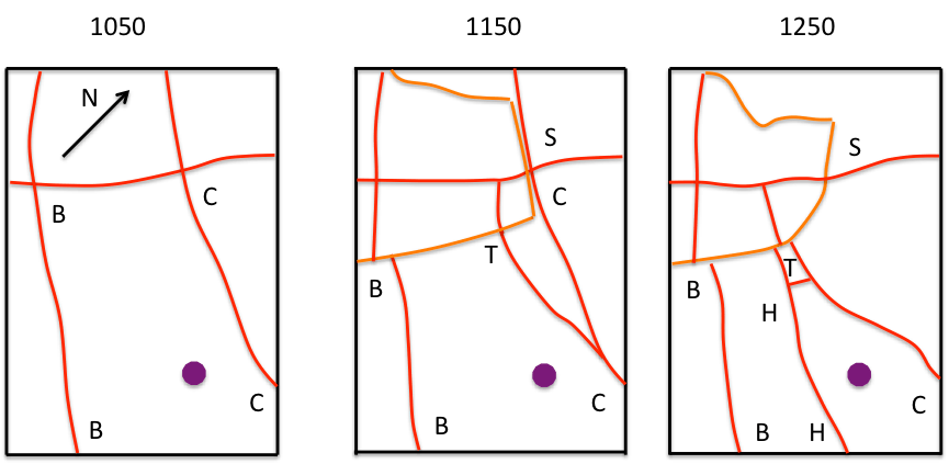
Figure 3. Roads in the vicinity of St. Michael’s

(Road identifiers the same as in figure 2. H – Sturgeon’s Hill / Rotten Row, S – Stowe Gate, T – Tamworth Gate. The edge of the burgh is given by the brown line)

Basset also looked in detail at the development of the city. In short, the city was a planned development, laid out by Bishop Roger de Clinton around 1125 to 1150 Figure 3a shows the roads around St Michael’s around 1050AD, with the same identification letters as in figure 2. Figure 2b shows the road layout inferred by Basset in 1150AD after the Burgh was laid out. It can be seen that a new road has developed from Road C (Burton Old Road) and heads to the Tamworth Gate (denoted by T). The old road continues to the Stowe Gate (S). By 1250AD the situation has changed somewhat. The old road to the Stowe Gate no longer exists (although it can even now still be traced by the lines of back gardens along part of its course. Road H (Sturgeons Hill / Rotten Row) has appeared and converges on the Tamworth gate and the diverted road C. At the gate there was an open area that was used as a market, and which ultimately became the cattle market. The diverted section of road C was eventually to become part of Trent Valley Road / Church St. at the bottom of St. Michael’s graveyard. The important point to appreciate is that over the course of this development, the area around St. Michael’s graveyard became increasingly constrained, both by Road H and by the diversion of Road C and the market area. It is quite possible that the size of the graveyard was actually reduced by these constraints.

Archaeology

There have been two archaeological excavations at St Michael’s in recent decades. The first was by Gould and Gould (1976) who cut a trench in he bank between the old and the new churchyard to see if there was any evidence of a churchyard enclosure, as is often found around ancient churches. There wasn’t. You win some and you lose some.

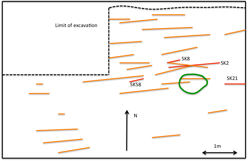
The second excavation was carried out in 1978 on the site of the new choir vestry (Wilson, 1981). A sketch of the excavation is given in figure 4. This was rather more profitable in terms of the archaeology as follows.

A single post pit, filled with sandstone fragments in the bottom layer.
49 complete or partial skeletons, mostly buried in the Christian manner with head to the west (so they would face their maker at the resurrection). There were two exceptions. Skeleton 21 was buried with its feet to the west, in a manner that would be suggestive of a priestly burial (so he would face his flock at the resurrection). The expected chalice and paten were not found, possibly because this skeleton was at the edge of the excavated area and it head was outside the area. Murphy’s law and all that. Alternatively Wilson suggests he simply could have been buried the wrong way round. Skeleton 58 was a crouched burial. Such burials are known from Palaeolithic times. In a Christian context they are most often dated from the Anglo-Saxon period. No independent carbon dating was possible. In addition skeletons 2 and 8 were of a woman and a small child – who possibly died during childbirth.
Five flint flakes from the Mesolithic period but in a secondary context; large quantities of building material from earlier churches, including 300 fragments of glazed medieval roof tiles; a range of different types of decorated floor tile; a sherd of Roman pottery; a halfpenny from the reign of George III and a silver penny from the reign of Richard II.

There thus seems to be some evidence of very early use of the Greenhill site, but precise dating was not possible.

Figure 4. The 1978 excavation

(There of excavation covers the area of the current choir vestry. Brown lines indicate burials with skull to the west. Red lines indicate specific skeletons discussed in the text. Green indicates the posthole.)

A personal postscript

There is a further quasi-archaeological point of personal interest. In 1822 one John Baker and his wife Anne (nee Woodfield) were buried in the churchyard at the location shown in figure 5. They were my great-great-great grandparents. I can find out little about them other than that they were very prolific in producing children (11 can be traced). They were one of the few of my ancestors to be able to afford a gravestone. St. Michael’s monumental inscriptions records the inscription as

2022 John Baker 17/9/1822 also Ann Baker

So it was probably not a terribly large gravestone. It has of course been moved as the churchyard has been tidied over the recent decades and I don’t know its location. If anyone comes across it at any stage please let me know! Further fascinating details of my family tree, the members of which were almost exclusively miners, ironworkers or agricultural labourers, can be found here.

Figure 5. Location of John and Ann Baker’s grave

References

Basset S (1981) “Medieval Lichfield: A topographical Review”, Transactions of the South Staffordshire Archaeological and Historical Society, XXII, 93-121

Basset S (1992) “Church and diocese in the West Midlands; the transition from British to Anglo-Saxon control”, Pastoral Care Before the Parish p. 13-40

Gould D, Gould J (1976) “St Michael’s churchyard, Lichfield, Staffs”, Transactions of the South Staffordshire Archaeological and Historical Society

James T (1998) “The development of the parish of St-Michael-on-Greenhill over 1500 years”, St Michael’s papers number 1, PCC of St Michael’s, Lichfield

Victoria County History (1990) ‘Lichfield: Churches’, in A History of the County of Stafford: Volume 14, Lichfield, ed. M W Greenslade (London, 1990), 134-155. British History Online http://www.british-history.ac.uk/vch/staffs/vol14/pp134-155

Wilson P (1981) “Investigations in St Michael’s and St Mary’s churches, Lichfield”, Transactions of the South Staffordshire Archaeological and Historical Society, XXII,

“That way madness lies” – the search for solar alignments in Lichfield

Introduction

A few years ago, whilst looking at some maps of the Lichfield area where I live, I was struck by the overall southwest / northeast alignment of the city, and wondered if this might hide some sort of topographical alignment based on midsummer sunrise (in the northeast) and midwinter sunset (in the southwest). The fact that the bronze-age ceremonial centre at Catholme was to the northeast of the city encouraged me in these views. Now seeing alignments of any sort from maps isn’t terribly well regarded by serious historians – those somewhat idiosyncratic types who spend their lives looking for “lay lines” connecting monuments of different types have rather made this sort of speculation somewhat less than respectable. And there is some cause for this suspicion, as alignments of different sorts can be found almost anywhere should one look hard enough. For instance I noted a few years ago that Borrowcop Gazebo, Lichfield Cathedral and Rugeley Power station were lined up very nicely, which I suspect doesn’t have much historical significance. But nonetheless these thoughts have stayed with me, and given that during the current lockdown situation I have time on my hands, I thought I would investigate this a little further. This blog post is the result. In the next section I outline how the directions of summer sunrise and winter sunset can be accurately calculated using some simple maths (readers who don’t like that sort of thing may care to pass over this section quickly). I then identify a possible midwinter sunset alignment from Catholme. Finally I speculate on what might be the implications of such an alignment,

Calculating solar alignments

Wood (1978) gives the following simple formula for calculating the azimuth (degrees from north) of the midsummer sunrise midwinter sunset

The site latitude is easily determined from geographical data. The elevation is the angle from the point of observation to the horizon over which the sun will set, corrected for the curvature of the earth and atmospheric refraction. The actual angle is easily obtainable from software such as Google Earth, and Wood (1978) gives values for the two corrections. The declination is the angle between the plane of the celestial equator and the terrestrial equator. The values of this angle for the midsummer sunrise and midwinter sunset have the same magnitude but different signs. The declination also varies with time, so the values from 4000 years ago differ from current values by about 0.6 degrees. This is quite important for the calculation and needs to be specified by a historically reasonable time being specified for the alignment in question.

The Catholme alignment

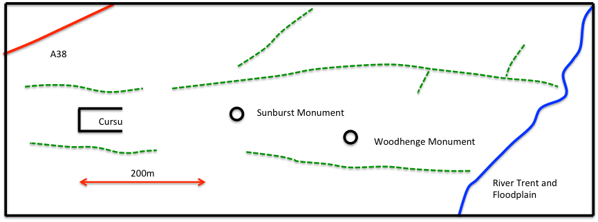
The first step in identifying whether or not there is a possible solar alignment is to identify the end points of such an alignment. So we begin with Catholme itself. The ceremonial complex is shown in figure 1. Essentially there are three monuments within the complex – a cursus dated to around 3000BC; a sunburst monument due east of the cursus, characterised by post holes radiating from the centre, and a Woohenge monument, characterised by concentric circles of post holes, to the east of the sunburst monument and slightly to the south. The Sunburst and Woodhenge monuments have been dated to between 2600 and 2400BC and remained in use for several centuries. There thus seem to be three possible starting points for the alignments, at each of the three monuments.

Figure 1 Sketch of the Catholme complex (Chapman et al, 2010)

But what of the other end of the alignment? In the first instance I expected this to be in the Lichfield area, but a study of the topography profiles (using Google Earth) on a south-westerly line from Catholme through Lichfield shows that Lichfield lies in a hollow and can’t be seen from Catholme. Also the horizon from Catholme is well beyond Lichfield in the Walsall Wood / Pelsall area. An investigation of maps of this area however revealed a very suitable location in Castlebanks (the site of an Iron Age Hill fort), a prominent hilltop that would have been on the horizon from Catholme and would act as a natural marker for observing the setting of the sun.

So as a first step, I calculated the directions from the three Catholme monuments to Catlebanks, simply using the longitude and latitude values for each of the sites. These are as follows, with direction measured clockwise from north.

Cursus to Castlebanks 225.7 degrees

Sunburst monument to Castlebanks 226.4 degrees

Woodhenge monument to Castlebanks 227.4 degrees

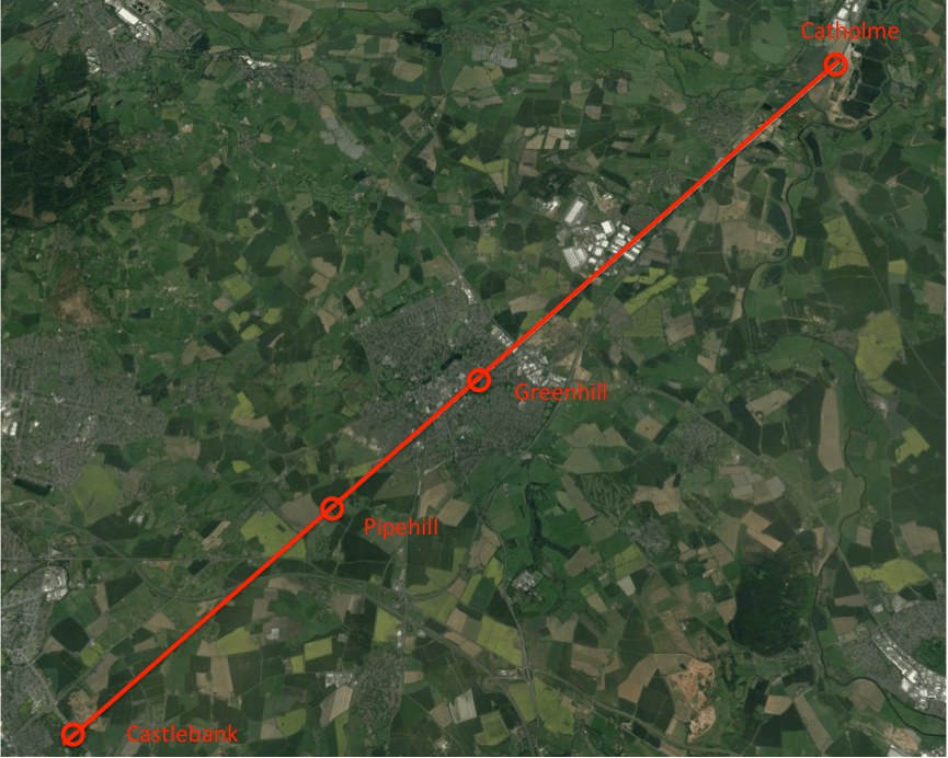
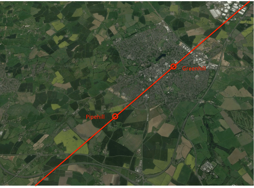
So there is a difference of around two degrees in the alignments from the various Catholme monuments. The next step is to find the direction of the midwinter sunset from Catholme around 2500BC. The latitude of that site is 52.74 degrees and the elevation can again be found from the profile produced by Google Earth. With the corrections specified by Wood (1978) this value comes out close to zero at -0.2 degrees. Wood (1978) gives a declination of – 23.98 degrees for 2500BC for the midwinter sunset. Putting these values into the above equation gives a value of 228.1 degrees for the midwinter sunset as seen from Catholme. This figure changes slightly to 228.0 degrees using the declination for 3000BC. Using the current value of declination, gives a direction of 229.1 degrees. Also of course there would be an offset of up to -0.5 degrees depending upon how the observer defined the sunset, and the particular topography that ultimately obscured it, giving the most likely value as being around 227.6 degrees. On this basis, the Woodhenge to Castlebanks line seems the most likely alignment. This is shown in the figures below. Figures 2 and 3 are Google Earth screenshots ands show the complete alignment and an expanded view of the alignment over the Lichfield area. Figure 4 is the elevation profile for the whole alignment. It can be seen that this line passes over Lichfield as expected, but its exact course is of interest. It passes over Greenhill (where the church of St Michael stands) and over the high ground at Pipehill, the source of the springs which provided water to Lichfield for many centuries. In fact from Carholme the midwinter sunset in 2500BC would have taken place over a line of hills – Greenhill in the foreground, the Pipehill ridge behind it and Castlebanks on the horizon. The midwinter sunset alignment here is so good, I do not think it can be accidental. The lining up of three prominent hills on a midwinter sunset alignment was probably just too good to miss for a Bronze Age priest who wanted to add another solar alignment to his ceremonial complex!

Figure 2 The Catholme – Castlebank alignment

Figure 3 Expansion of the map of figure 2 over the Lichfield area

Figure 4 Elevation profile of the Catholme – Castlebank alignment

Speculations on meaning

Clearly Catholme included solar alignments from its earliest date – the east-west axis of the cursus, with the Sunburst monument on the same alignment, would give two spring / autumn equinox alignments. The Woodhenge monument thus seems to have been positioned to create a midwinter sunset alignment with Castlebanks. What the ultimate purpose of these alignments were is of course impossible to know – they may have been purely for calendar purposes, or may have had a deeper cultic aspect. But from the perspective of a current Lichfield resident, I would like to ask if the Lichfield area were in any way, other than an accidental one, part of this overall scheme?

Now Pryor (2003), based on a study of a wide range of pre-Roman sites, identified the following characteristics that indicate the ritual use of such sites.

Solar or lunar alignments.
Rivers, marsh or open water, which has been used for votive offerings of weapons and other utensils, sometimes with causeways in to or across the body of water.
The proximity of barrows or other burials.
A distinction between the “domain of the ancestors” identified by “hard” stone monuments, and the “domain of the living” identified by “soft” wooden henges or monuments.
The usage of the site by many groups or tribes, as a communal meeting point.

Now let us address each of these issues in turn for the Lichfield area.

Clearly the Lichfield area meets the first of these criteria – as part of the longer Catholme – Castlebank alignment and also with Greenhill and Pipehill being on that alignment and having an internal alignment of their own.
In terms of rivers and bodies of water, there are clearly springs on both Greenhill and Pipehill, and the centre of Lichfield was likely to be quite swampy at the confluence of the Leamonsley and Trunkfield brooks. Both neolithic and bronze age axeheads have been found in the area, although the precise locations are not known. Such artefacts have been known to be ritually deposited at other sites (Carver, 1981).
There are a number of prominent barrows in the area, and in particular Offlow to the south, and possibly Borrowcop to the south east.
There is no archaeological indication of stone monuments from the bronze or iron ages in the Lichfield area, but there is of course the historical association of Greenhill with the rituals of death – the large graveyard at St Michael’s church and the dedication to the Christian “psychopomp”, the collector of souls. But these indications come from 2000 years after the Woodhenge monument was last in use.
Similarly with regard usage of the site for communal gatherings, Bassett (1981) has shown that in the pre-Roman era, Lichfield was the centre of an extensive trackway system linking a range of communities in the area. But again this reflects a later age.

From this it can be seen that there are perhaps some indications that the Lichfield area fulfils some or all of Pryor’s criteria for a cultic site set out above, including the existence of the solar alignment, and may be of importance as a cultic site from early times. But of course, as with all such speculations, final proof is impossible.

References

Ancient Monuments UK (2019) https://ancientmonuments.uk/115453-hillfort-known-as-the-castle-fort-at-castlebank-plantation-aldridge-north-and-walsall-wood-ward#.Xo8tmi3MxzA

Bassett S (1981) “Medieval Lichfield: a topographic review”, Transactions South Staffordshire Archaeological and Historical Society, XXII, pp 93-121

Carver M G H (1981) “The archaeology of early Lichfield: an inventory and some recent results” Transactions South Staffordshire Archaeological and Historical Society, XXII, pp 1-12

Chapman, H, Hewson, M & Watters, M (2010) “The Catholme Ceremonial Complex, Stafforshire, UK”, Proceedings of the Prehistoric Society, London. 76, 135-163, 10.1017/S0079497X00000487

Pryor F (2003) “Britain BC”, Harper Collins, London

Wood J E (1978) “Sun, moon and standing stones”, OUP

Corbyn’s Hall from above

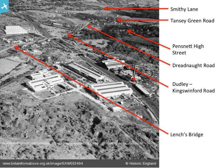
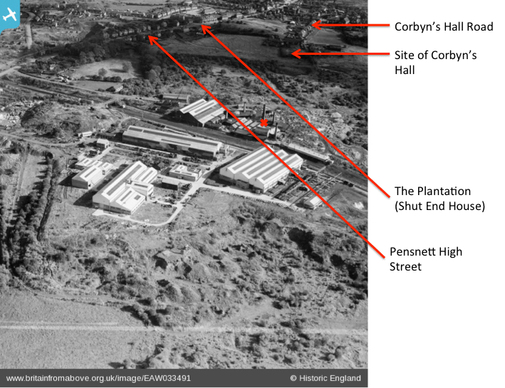
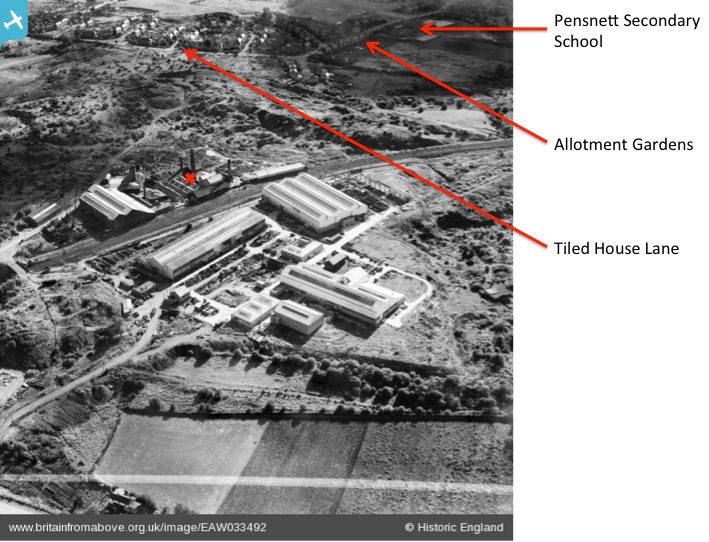
The “Britain from Above” archive contains a huge number of aerial photographs covering the entire country. These are usually arranged in sets of photographs concentrating on a particular notable landmark, and they give a huge amount of detail of the area around the site. Low-resolution photos can be downloaded and used on websites, and a simple free registration allows the reader to zoom in to small parts of the photographs for amazingly detailed views. When a search is made for Kingswinford, two sets of photographs appear – one is a set of six photographs of “Woodfield House and its Environs, Kingswinford, 1939” and the other a set of nine photographs of “Gibbons (Dudley) Ltd Silica Works at Corbyn’s Hall, Kingswinford, 1950”. It is with the second that this blog post is concerned. I will post some of the low-resolution photos taken as the plane flew around the site and label them with information contained on the large scale Ordnance Survey map for the 1950s from Edina Digimap. Taken together they provide us with a glimpse of the Corbyn’s Hall area in the 1950s and also, if one looks carefully, at the neighbouring villages of Kingswinford, Pensnett and Bromley.

Gibbons (Dudley) Ltd

The firm was founded in 1834 by Benjamin Gibbons, who is discussed at length in Kingswinford Manor and Parish, using high-grade fireclay to make bricks. They manufactured refractory products – firebricks, cements, concretes and plastic refractories. The main works was at Dibdale, Lower Gornal with additional works at Cooper’s Bank and Corbyn’s Hall, Pensnett. The Pensnett works was just one of the industrial concerns that grew and prospered on the Corbyn’s Hall estate that came into the ownership of the Gibbons Family in 1780. These included coal mines, iron and steel works and brick works. The map from the 1950s indicates a brick works at the centre of the site, with a number of chimneys, which was presumably the Sillica works, but also a large steel works and numerous disused coal and ironstone pits. In all the photographs that are used, the tallest chimney at the works will be marked by a red cross as a point of reference for the reader.

Looking northeast

We begin with the view looking northeast over the site, given. Here the relevant photograph is given twice. The first highlights the roads in the area – the Kingswinford-Dudley Road, Dreadnaught Road, Tansey Green Road, Smithy Lane and Pensnett High Street. Lench’s Bridge is also shown. This was built to span the Stourbridge Extension Canal. Little can be seen of this canal by 1950, it having been abandoned several decades earlier, although I will indicate its course in later photographs. The second photograph shows the various industrial concerns in the area, mainly distributed along the Wombourne Branch Railway (at this time still part of the through route for goods trains from Stourbridge to Wolverhampton). Just south of the main road is the site of Pensnett Halt, one of the stops on the short-lived passenger service on the line in the 1920s. On the Corbyn’s Hall site itself the brick works and steel works can be seen, the former being marked by a red cross as mentioned above, together with a number of old colliery workings. On the northern side of the Dudley – Kingswinford Road there are the Dreadnaught tile works and Stourbridge Refactories, both rail connected. The sawmill just to the south of the road has a long history and it can be traced back in census records to the 1880s at least. One of the most obvious features of the photograph, that will be observed on all those that follow, is the large area of waste ground around the site – caused by a century or more of coal and ironstone mining and other industrial use. This area, with all its hidden dangers, was the playground of my youth.

Looking east

The next photograph shows the view looking east over the site. In the background we can see Pensnett High St, the large house known as the Plantation, which was formerly known as Shut End House, the residence of Ben Gibbons himself. The photo also shows the site of the original Corbyn’s Hall which suffered badly from subsidence due to the mining activities and was demolished in the early years of the twentieth century.

Looking southeast

The next photograph swings round further and looks southeast. At the top of the photograph Tiled House Lane and its numerous cul-de-sacs is clearly seen, together with a region of allotments and Pensnett Secondary Modern School. The large area ofwaste land between Tiled House Lane and the works is very obvious.

Looking south

The next photograph looks due south towards Bromley, with Bryce Road, Bromley Iron Works and the disused New Bromley Colliery in the distance. I include on this photograph, and the following two, the line of the abandoned Stourbridge Extension Canal. It can be seen that the steel works is effectively built over the line of the former. The canal had a number of short branches. One of these served the Corbyn’s Hall old iron works which was on the left of the picture, and would have left the main line somewhere under the modern works, and gone under the railway line. The other was the Standhills branch, which left the main line somewhere around the top of the photograph and followed a large loop to the west.

Looking west

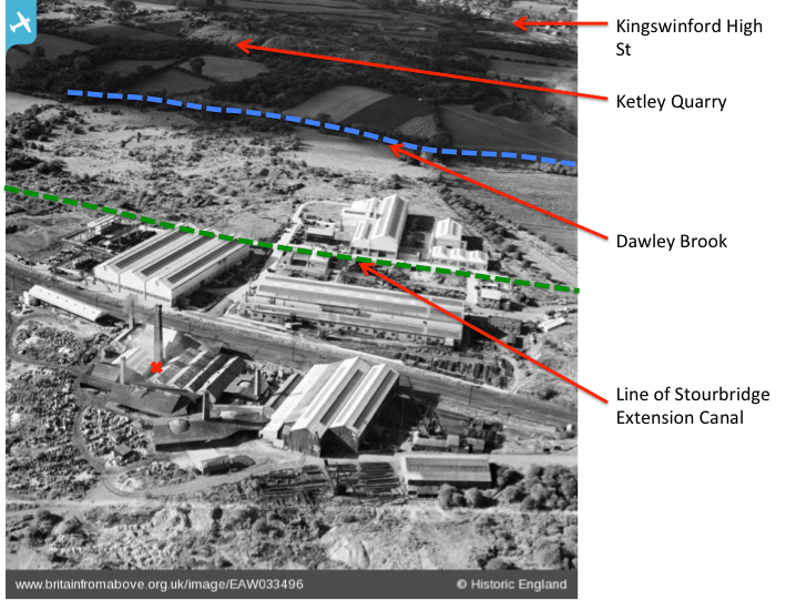
This photograph looks due west towards Kingswinford in the background. I have indicated on it the line of the Stourbridge Extension Canal, and also the line of Dawley Brook. The latter marks the bottom of the steep slope down from Commonside in Pensnett towards Kingswinford. The original Corbyn’s Hall estate extended well to the west of the brook. On the Fowler map of 1822, this brook had a number of pools along its length – which were possibly the remains of mill pools or ornamental features.

Looking northwest

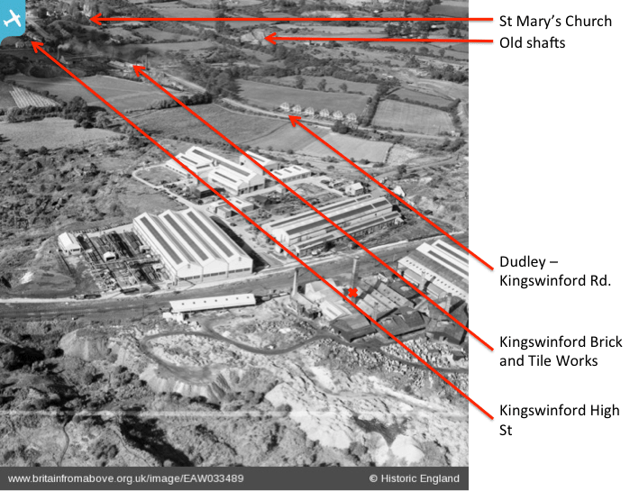
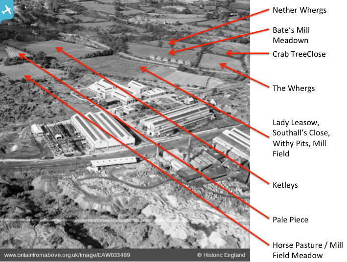
The last photograph, looking northwest, is repeated three times. On the first the Dudley –Kingswinford Road is again labeled, together with the Kingswinford Brick and Tile Works, St Mary’s Church and the old shafts and spoil tips of Shut End Colliery. The second again shows the lines of the Stourbridge Extension Canal (on both sides of Lench’s Bridge) and the Dawley Brook, and also shows the line of the original Kingswinford Railway (of Agenoria fame). The third shows the names of some of the surviving fields. These can be linked back to the 1822 Fowler Map of the area, and also earlier 18^thCentury maps of the Corbyn’s Hall Estate. Their essentially rural names speak of a very different age. Some of these names indicate the presence of mills along the Dawley Brook. I find it remarkable that they were able to survive in an identifiable form as late as the 1950s.

More detail

As mentioned above, much more detail can be seen by zooming in on the photos on the Britain from Above site. It is tempting to reproduce screen shots of these views here, but I don’t think this would meet the license conditions. But I would urge interested readers to have a look. The specific views that intrigue me are on the “Looking east” photo, where one can see the large open cast area just west of Tansey Green (close to the old Shut End Methodist Chapel), the Birds Meadow school, and the back of the Independent Methodist Chapel on Commonside (the successor to the Shut End Chapel, and the one I attended as a child); and on the “Looking southeast” photo the close up of houses in Tiled House Lane – including the one where I spent the first 18 years of my life. Do take a look!

Cornyn’s Hall today

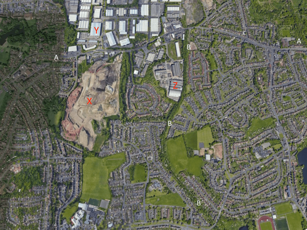
Finally, following a request from Tony Garratt (see comments), the figure below shows the area in 2020 (from Google Earth). I have marked the Kingswinford to Dudley Road (A-A-A) and the Wombourne Branch railway line (B-B-B) for comparison with the other photos. The picture is dominated by Ketley Quarry (X), the Pensnett Trading Estate (Y) and the industrial premises on the part of the site shown in the photos above, to the west of the railway line (Z).

Some thoughts on Family Tree studies

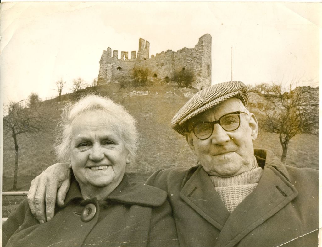
Alice and Sidney Baker – my paternal grandparents

A salutary lesson

Over perhaps the last ten years, I have spent some of my spare time researching my family tree, in a fairly ad hoc and disorganised way, but I had nonetheless built up a considerable set of information, and one or two branches on my tree reached back to the 1650s. In recent weeks, having a little more time because of retirement and enforced isolation, I have been looking again at all the information in a hopefully more systematic way. I have posted the results of my endeavors at the Baker Family Tree on my website. During this reappraisal, I have tried to make sure that all I include is properly sourced in census, birth, baptism, marriage or death records. I did however find that, in my enthusiasm to push my tree back as far as possible, I had previously used some unsourced family tree material found on, for example, Ancestry Public Member Trees. When I came to check where this material came from, I could not actually find any proper sources in a number of cases, and I have had, regretfully, to remove such material from my tree, and in doing so have lopped of a few quite long branches. Looking at the various public trees, I am clearly not the only one who has done this, with some of the unsourced material I initially used being repeated in a number (and sometimes a large number) of family trees. The temptation to do so is obvious as it represents a quick way of identifying ancestors, but it retrospect it was not the wisest thing to do.

The Baker Family Tree

That being said, the whole affair has made me think a little more deeply about the accuracy and quality of information that is available to build up family trees. As a result, I have carried out some simple analysis using my own tree to try to investigate these issues a little further. Before going any further however, I need to make clear the characteristics of this tree, as to some degree these determine what follows. Very broadly my ancestors, as far back as I can trace them, were either miners, ironworkers or industrial or agricultural labourers of some description – in other words at the bottom of the social scale. The tree is centred on a region at the western edge of the Black Country, and by and large my ancestors come from within 30 to 40 miles of there, as far back as I can trace them. Some of the branches of the tree can be traced back to the seventeenth and eighteenth centuries in places where there are comprehensive surviving baptismal and marriage registers – in particular in the Anglican churches in Lichfield, and the non-conformist churches in Shifnal in Shropshire. On my website, I present my tree as four separate sub-trees, beginning with my grandparents – the paternal grandfather tree, the paternal grandmother tree, the maternal grandfather tree and the maternal grandmother tree. I label my grandparents generation as generation 1, their parents as generation 2 and so on. The tree concentrates on my direct ancestors, although I do give details of the children of direct ancestors where I have found this information. More could be done in this regard. The other very specific oddity of the tree is that both my father’s surname and my mother maiden name was Baker, so there are two, independent, Baker sub-trees.

Generation length

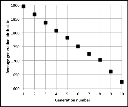
Firstly I looked at the average birth / baptism dates for each generation, using the information for each member of the tree that was available. Birth dates are plotted against generation number in figure 1 below. Basically it shows that, on average, the generations are spaced at around 25 to 30 year intervals – which seems reasonable, given that most of my ancestors married at around the age of 20 and those who bred successfully continued to doing so into their forties.

Completeness

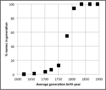
Secondly I looked at the completeness of the tree. In each generation there are a theoretical maximum number of individuals – 4 in generation 1, 8 in generation 2, and up to 4096 in generation 10. Figure 2 shows the percentage of this maximum number that I have identified in each generation. For convenience I plot this percentage against the generation birth date. It can be seen that this percentage remains high for birth dates back to around 1800, then drops rapidly, and remains at a low level as far back as the trees can be traced in the seventeenth century. The major fall off in the completeness of the tree around 1800 is due to the fact that individual born before that rarely appear in the censuses from 1841 onwards, and that the coverage of parish and non-conformist registers is somewhat patchy before this date. Information finally runs out around 1630 to 1650, before which the parish records were all but non-existent. For trees such as mine these two dates represent significant information horizons. For those with ancestors somewhat higher up the social scale there may well be other sources of information available that allow trees to be pushed back further in time. Taken to its extreme, the House of Windsor can trace its pedigree back to the early royal houses of Wessex, Mercia, Dal Riada and the Picts etc. Indeed, if one believes some genealogies this pedigree can be traced back further to Woden, although the source information for that is probably not readily available.

Quality

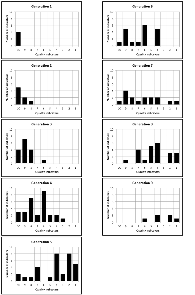
I then looked at the quality of the information for each individual in the tree. I used a scoring system with one point allocated for each of the following pieces of information.

Birth / baptism year
Birth / baptism location
Marriage year
Marriage location
Death year
Father’s first name
Mother’s first name
Mother’s maiden name
Spouse’s first name
Spouse’s surname

Whilst the list is to some degree arbitrary, in my experience the more of these details that are known about an individual the more confident one can be about their place in the tree. There are thus a maximum of ten points for each person. Applying this to my tree, one can draw histograms of quality scores for each generation, and these are shown in figure 3 below. Generation 1 has four entries, all of which have maximum scores. The number of entries increases through generations 2 to 4, but in general the quality of information remains high, although it is beginning to spread out by generation 4 with some low scores. Generation 5 is however distinctly different, with a large number of individuals with low quality scores. This corresponds to the fall of in the number of identifiable individuals in figure 2 for this generation with an average birth date of 1780, and the low scores represent individuals whose line can be traced back no further. Generations 6 to 9 then show a wide spread of scores, with high scores for those branches that are well documented, and low scores for those branches that are coming to an end. The high scores become fewer and fewer as the generation date approaches the early limit around 1630 to 1650.

This raises the question as to whether it would be sensible to impose a confidence limit on individuals in tracing back family trees. My own feeling is that if the quality score for an individual is 3 or below, then it would be wise to stop the tree this point, rather than making speculative identifications from the record for earlier generations.

Ambiguity

As I noted above most of my ancestors were very unadventurous in terms of where they lived and all came from a quite restricted area. This same tendency can be seen in the names they chose for themselves. There are 21 different first male names in my tree, with the top four being John, William, Joseph and Thomas (in that order), accounting for 65% of the total. There are slightly more female names – 27 in total with the top four in order being Mary, Ann, Hannah and Sarah, which account for 47% of the total. This is very consistent with the analysis of the names in the Book of Reference to the 1822 Fowler Map of Kingswinford in Kingswinford Manor and Parish. Here the top four male names were the same as in my tree, and in the same order and accounted for 55% of the total. The top four female names in my tree are all in the top five of those in the Fowler Book of Reference, although not in the same order, and together they make up 57% of the total. This concentration of names is matched throughout the area over the period from 1600 to 1900. Also “Baker” is a common name with two Baker families being represented in my tree with perhaps half a dozen other Baker families in the records in the immediate vicinity, and many of the other names in the tree are equally common. Putting these two facts together, it is easy to see that in a number of cases, there is significant ambiguity in identifying individuals in the record. The name “John Baker” was particularly difficult in this regard – there were a lot of them about. It is this ambiguity that brings many branches of the tree to an end. I have taken the view that if there is there is more than one candidate for a particular place in the tree, and there is no strong supporting evidence for choosing one above the other (such as, for example, birth / baptism location) then it is best to make no identification until further evidence can be found.

Final thoughts

Finally, can my reflections above, based on my own, really very specific , family tree, be generalized in any way? I think a number of fairly general points can be made.

The two information horizons I identified will be generally true for all those trees without a high status component, and all such trees are likely to thin when the generation birth dates are before 1800, and to run out completely around 1650.
The concept of quality of information might be useful to those researching trees, in identifying an appropriate place to stop each branch.
Very great care should be taken with ambiguous situations – there is little point in pursuing a branch back in time if there is a significant probability that one link on it may be incorrect.

The Shut End Primitive Methodist Chapel. Part 3 – Ministers and families

Part 2 of this post can be found here.

The Baptismal Register gives details of those ministers who baptized the children. These can be expected to be in two categories – members of the church who held a position of authority of some form and conducted services – perhaps stewards or trustees; and preachers from the local Primitive Methodist Circuit. In total 151 baptising ministers are listed (although the variable forms of the names may mean this is an overestimate), with most officiating at just a few baptisms. The five most common baptizing ministers are shown in table 6 below.

The census returns in principle allow a little more information to be gleaned for these ministers. For one of them – Robert Bowen – there is however no obvious candidate in the census record. Of the others, William Dudley was born in 1817 in Oldswinford and in 1861 he is listed as a tailor and draper in Kingswinford. Samuel Kendrick was born in 1811 in Ketley in Shropshire, lived in the Smithy Lane area and is listed as a miner. Abraham Dodd was born in 1844 in Oak Farm and worked as a miner. He was the son of another Abraham, a miner from Wombridge in Shropshire. There are a number of Joseph Homer’s in the census record, born around 1835 to 1845, so it is not possible to be precise concerning his birth or residence, although all of the possible Joseph’s were either miners or labourers.

The longevity of the ministry of all in table 6 would suggest that they were all members of the congregation itself – indeed in the case of Sam Kendrick and Abraham Dodd, their families can be traced in the baptismal entries themselves. It is likely that many of the others who performed just a few baptisms were circuit ministers. Only two such can be identified with confidence by their appellation – Rev R Brewen in 1861 and the Rv J Hawkins from 1881 to 1884. Dood (1883) draws attention to another possibility – Henry Higginson – and says that he was nicknamed the Roving Ranter. Unfortunately the census records reveal no more about him, which is the greatest of pities, as the name suggests there are stories to be told.

Two further points arise – firstly the ministers in the local congregation all shared the same background as those to whom they ministered, as manual workers or small shopkeepers. Secondly the link with the Shropshire coal field is obvious. In KMAP I described the society in Pensnett in the 19^thcentury as a migrant society, with a considerable population influx, particularly from the Shropshire area.

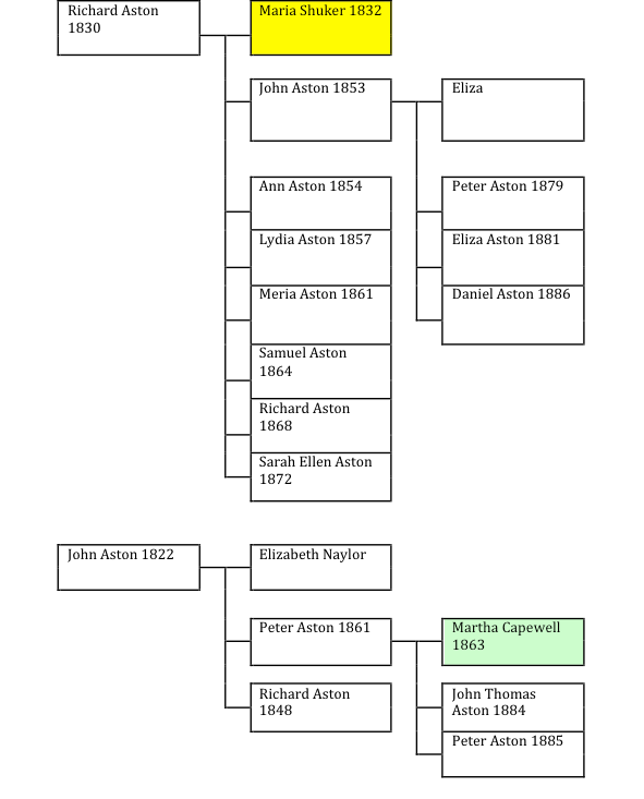
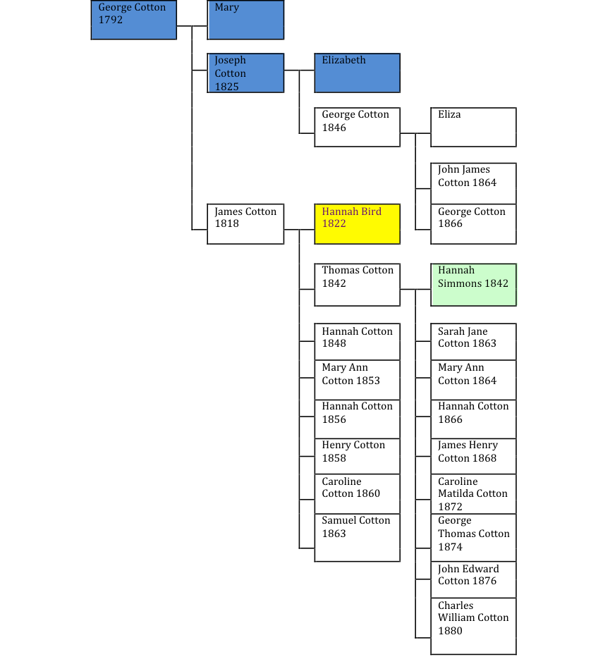
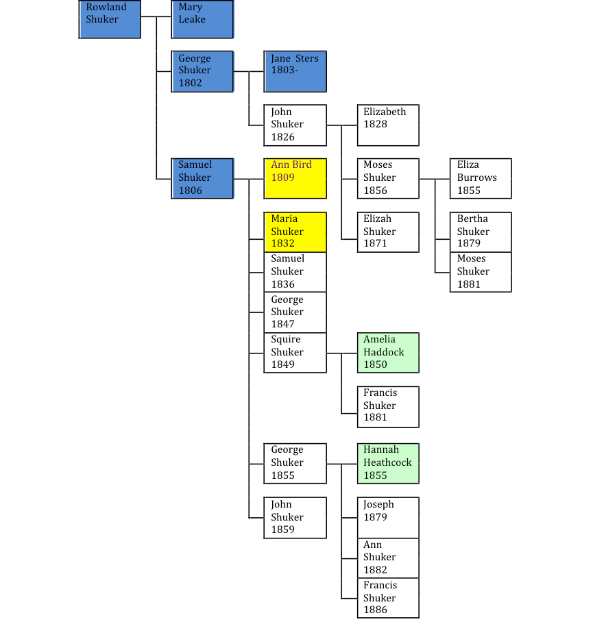
To fully describe all the families and individuals mentioned in the register is of course not possible, and its primary use in this regard will be by those researching family histories. The approach I take here is to consider in some detail just three families, who between them were involved in 46 baptisms over the course of the 42 years of the register. These are the Astons, the Cottons, and the Shukers. The family connections for these three families are shown in figures 3, 4 and 5 below. In these figures the following conventions have been adopted.

Those individuals with no shading on their entry appear directly in the register either as parents of as the child being baptized.
Those shaded in green indicate membership of families that appear elsewhere in the register.
Those shaded in blue indicate individuals who have been identified through census / BMD searches, usually from generations earlier than those in the register, that connect some of the register entries together.
Those shaded in yellow indicate linkages between the three families.

Note that these trees only show the names of individuals in the register or those who link the various individuals together. Many of the families in these figures can be shown through census records to have other children who do not appear in the register for one reason or another.

First consider the Aston tree shown in figure 3. Three generations of the family appear in the register. Those in the first generation – John (1822) and Richard (1830) were probably brothers, but their parents are elusive in the record. The earlier generation comes from the Dudley area, and the later generations lived in the Tansey Green and Commonside areas. Without exception all those in the register were manual workers throughout their lives. Richard (1830) married Maria Shuker (1832), the first of the inter-family connections that we can identify.

The Cotton tree in figure 4 covers four generations. George (1792) (not in the register) came from the Wombridge area of Shropshire (near Oakengates and Wellington), and the two distinct families of the Cottons were his descendants, migrating to the Kingswinford area in the early 19^thcentury. James (1818) and Hannah Bird (1822) also come from the same area. Hannah is the second of the family interconnections – see below. After the family moved to the Pensnett area, they all lived around Shut End / Coopers Bank / Tansey Green. Without exception, all the males mentioned in the register were miners.

The third tree in figure 5 is that of the Shukers. Here 5 generations are shown, with the latter three appearing in the register. The early generations were again from the Wombridge area. Samuel Shuker (1806) married Ann Bird (1809), the elder sister of Hannah in figure 4. The Bird family was again from Wombridge. One of their children, Maria (1832) married into the Aston family (figure 3). The later generations lived in the Shut End / Tansey Green / Commonside area and were mainly labourers, but one or two were skilled manual workers.

These three trees can only of course represent a snapshot of a small section of the register, yet they do show the interconnectedness between the families and other families who attended the Chapel, and their common roots. Other families could of course be considered – such as the Dodds from Shut End and Tansey Green (12 baptisms), or the Greenaways from Coopers Bank (19 Baptisms), both of which had those in leadership positions in the church – Abraham Dodd (mentioned above) baptizing in the 1870s and 1880s, and Christopher Greenaway baptising in the 1880s. The significant point remains the same however – the lack of social and occupational mobility for such families.

The Shut End Primitive Methodist Chapel. Part 2 – The Baptismal Register

Part 1 of this post can be found here.

The typed transcript of the Baptismal Register of Dodd (1983) is a copy of a handwritten transcript, that has itself been significantly amended. This was in turn a copy of the original register. The Baptismal entries from 1845 to 1887 are given, with the following information.

Date of baptism
Christian name(s) of baptized child.
Christian name(s) of father and mother, and surname
Address – usually given by a broad area location
Occupation of father
Name of officiating minister
(Date of birth of child)

In total there were 777 entries over the period of 42 years, with 514 different couples represented. The Register can thus be seen to contain a great deal of potentially interesting information. However, it must be admitted that that the typed transcript of the register is a bit of a mess – which either reflects the original register, or may be partly due to its transmission history. Entries are not always in the correct date order, with some being significantly displaced. Names on the original were clearly difficult to read, and some of the guesses thus made are meaningless. The spelling is in general variable, which probably reflects the abilities of the officiating minister in transcribing names given orally.

To analyse the register in detail, I transcribed all the entries to an EXCEL spreadsheet, which was not one of the more exciting experiences of my life. To enable the data to be ordered to reveal its various aspects more clearly, some cleaning up was needed. This involved adopting common spellings for addresses, occupations and names. The latter had to be done with care, so as not to use essential information, but most name changes were trivial – for example to standardize on “Henry” rather than “Henery” or “Henary”. In other places a greater degree of interpretation was required. Whilst these changes may have resulted in minor errors that affect the statistics presented below, these should not be significant.

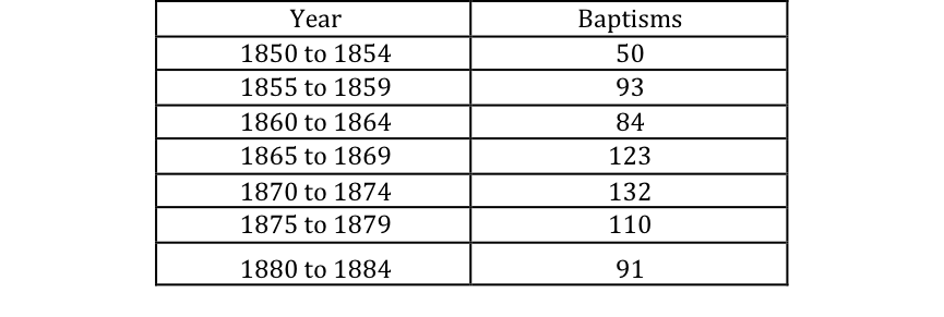
Table 1 shows the number of baptisms in five-year periods. It can be seen that these increase from 50 between 1850 and 1854 to a maximum of 132 between 1870 and 1874 i.e. from 10 to 26 / year on average. After that there is a slight fall off. KMAP shows that the population of the Shut End area followed a similar trend, peaking in the 1860s and then decreasing, and whilst the number of baptisms possibly reflects this, it also reflects the age distribution of the chapel congregation. Baptisms usually took place between 2 and 4 weeks after birth, but there were exceptions. For example, sometimes double family baptisms are recorded in the register. Whilst a few of these were baptisms of twins, for most of those where children’s birth dates are given, they are for a baby and an older sibling who had clearly missed out on baptism after birth for one reason or another.

Table 2 shows the number of baptisms by area of residence. To compile this table, the register entries have been consolidated somewhat – for example in the few cases where streets are given, these are included in the relevant area. In the table, the Pensnett area refers to the area of the new developments, mainly centred on the Hollies area, but extending as far west as New / Swan St. It is not clear to me how Shut End and Tansey Green were distinguished by residents, and there may well be some confusion between them. These uncertainties aside the vast majority of baptisms were of those in the 1845 ecclesiastical parish of Pensnett (Pensnett, Commonside, Shut End, Tansey Green and Bromley – 83.1% in total) and most of the rest from closely surrounding areas (Kingswinford, Coopers Bank, Oak Farm, Brockmoor, Brierly Hill and Wordsley – 13.8%). The remaining entries were wide spread, from as close as Dudley to as far away as Wigan, and probably indicate married children returning home for the baptism of their child at their home chapel.

**Table 2 Baptism entries by area of residence**

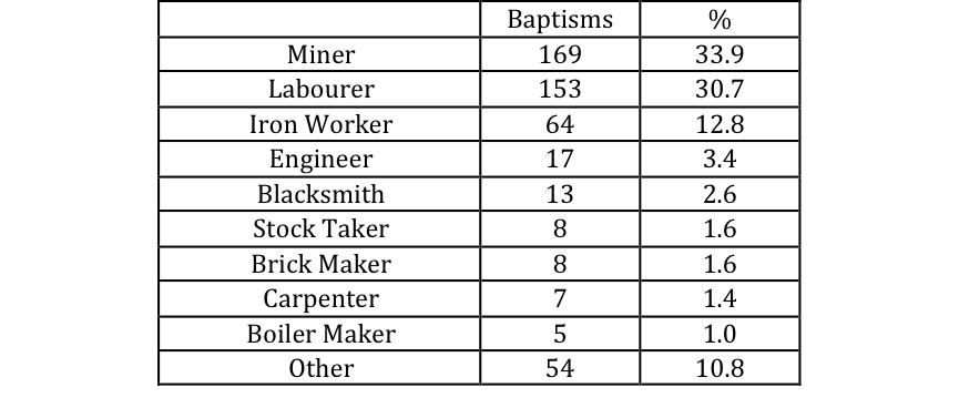
Table 3 shows the Register entries grouped by father’s occupation. Here again some cleaning of the data was required. The major change was to re-label a range of entries as “Iron Workers”. These took on a large variety of forms including moulder, furnace man, roller and puddler. Some of these, particularly the latter, were regarded as highly skilled jobs. The “other” category includes trades such as groom, keeper, horseman, boat builder, shoemaker, grocer, butcher, with a very small number classified as managers or clerks. It can be seen that the majority of the entries are for fathers who were miners or labourers, whilst almost all of the others would be working in or servicing the various industries listed. The labourers could be working in any of the other industries included in the list.

Now to some degree these figures will reflect the fact that the fathers of those baptized were relatively young and unskilled, and thus more likely to be labeled as labourers than their elders, but nonetheless they do show that the congregation at the chapel were overwhelmingly manual workers of various skill levels.

**Table 3 Baptismal entries by father’s occupation**

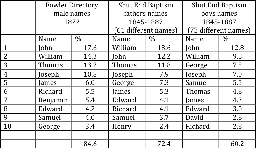
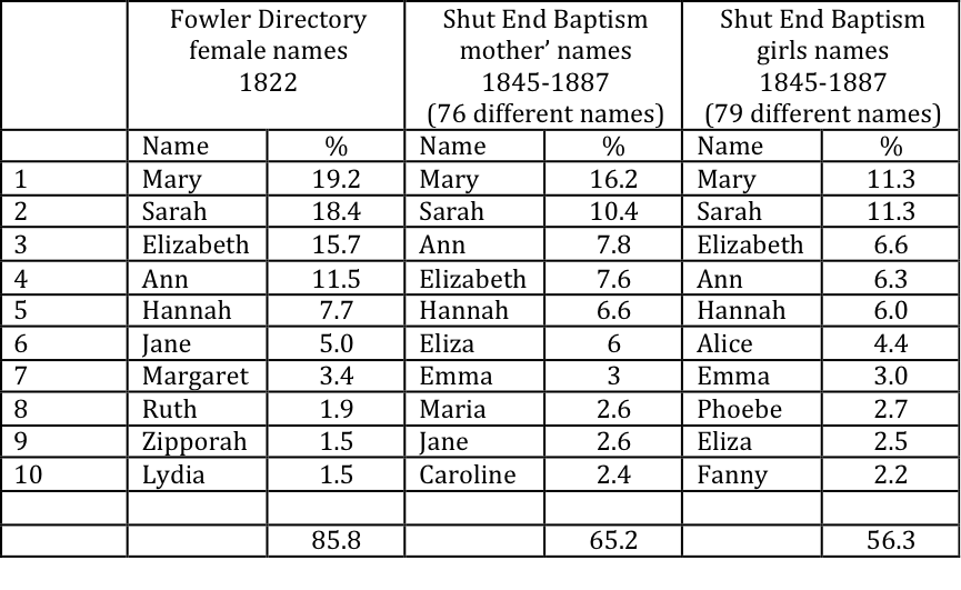
The baptismal registers of course give a very great deal of information concerning names – both Christian names and surnames. However this aspect of the register data is most difficult to analyse because of the huge variability in spelling, and a lot of cleaning of the data was required to put the most common names into a common format so that the data could be ordered and searched. The results of the analysis are shown in table 4 for male names and table 5 for female names. Each table shows the most common ten names and their percentage of the total from the following sources.

The Fowler 1882 map directory for the whole of Kingswinford parish (as included in KMAP).
The names of the mothers and fathers in the Baptismal register.
The names of the children in the baptismal register.

This thus represents three different time slices – the first reflecting names given between around 1780 and 1820, the second for the period between approximately 1820 and 1860, and the third for the period between 1845 and 1885. The second and third thus overlap somewhat.

Consider first the male names in table 4. The most striking thing is the similarity between the three lists, with most names occurring in all three. Benjamin, Richard and Samuel become less popular over the years, whilst George moves up the popularity list. Overall the top ten names contribute 85% to the total in 1822, but only 60% between 1845 and 1885, reflecting the fact that whilst that outside the most popular names, there was an increasing variability. For both the father’s and the son’s names, there was a consistent use of Old Testament forms, some more obscure than others. There were also a few oddities: from 1871, Lord Dando, son Mark and Caroline Dando of Pensnett, Blacksmith; from 1849, Squire Shuker, son of Samuel and Ann Shuker of Shut End, Engine Worker; and from 1860, Theophilus Hadduck son of Benjamin and Meriah Hadduck of Commonside, Forgeman.

The female names in table 5 show something of the same level of stability for the top 5 names, but thereafter the names in the list are very variable. In 1822 the top 10 names contributed 86% to the total, but for the baptized girl’s names, this figure fell to just 56%, indicating again a greater variability as the years go by. This trend seems to be more pronounced amongst the female names, perhaps indicating a greater influence of prevailing fashion, although it is probably best if I, as a male, say no more here. Of all the names the most variable in spelling was Maria and its variants – Mariah, Meria, Meriah and Marieh. Whilst they all obviously refer to the same name, the large number of occurrences of these variants suggests a variability in the way that they were pronounced – and thus recorded in the register. Again there were some oddities: in 1865, Tryphena Wassell, daughter of John and Sarah Wassell of Bromley, Brickmaker; in 1868, Ursula Adelaide Danks, daughter of William and Caroline Danks of Pensnett, Roller; in 1874, Adelaide Amos, daughter of John and Pamela Amos of Tansey Green, Miner. The name Adelaide seems to have been taken from Queen Adelaide, the wife of William IV.

In Part 3 of this series of posts I will consider in more detail the ministers of the church and the church families that can be found in the register.

The Shut End Primitive Methodist Chapel Part 1. Introduction and the chapel building

This is the first in a series of three posts concerning the Shut End Primitive Methodist Chapel in Pensnett, and in particular the period from 1845 to 1887. In this first post I will consider the physical nature of the Chapel itself and the activities that went on there. In the second and third posts I will discuss the very informative Baptismal Register for that period. It will be seen that this gives a wealth of information on the members of the chapel, their families and occupations. Nearly all of them were at the bottom of the social scale as labourers and miners, and the register allows their lives a little more visibility than would normally be the case.

Introduction

The Shut End Primitive Methodist Chapel is described in Kingswinford Manor and Parish (KMAP) as follows.

The other (Primitive Methodist) was the Shut End Methodist chapel, the history of which begins in 1832. The Chapel was situated on Tansey Green Road, and consisted of a Chapel Building and a Schoolroom. Directly behind it was the Shut End Pit, and there were later to be subsidence problems due to this. The first services were held in December 1832, and by 1836 meetings of some sort were also being held in Commonside and at Shropshire Row in The Oak……..The 1851 Religious Census records morning / afternoon and evening congregations of 110, 134 and 120 respectively, with 120 sittings provided, and in 1887 there were over 250 children in the Sunday School and 20 teachers. The Church also operated its own Friendly Society – the Shut End Primitive Methodist Economic (Sunday School rooms) with 54 members in 1878, and assets of £200. …….In 1861, the minutes of the Trustees of the Primitive Methodist Church on Tansey Green reveal an offer for the purchase of the building from the proponents of the Dudley and Bridgnorth Railway, part of the Welsh and Midland Counties Junction Railway – a line that was never given parliamentary approval and about which little detail is available……Over the years the building continued to deteriorate and there were repeated moves to persuade the local Primitive Methodist circuit to purchase land for a new chapel. Matters came to a head in the early 1890s when the congregation purchased land for a new chapel on Commonside themselves and were expelled from the circuit. It seems that payment of the quarterly circuit fees were also an issue at the time (Wesley History Society, 1961). In 1893 the original building, which by that time was badly in need of repair, was finally sold and the new Independent Methodist chapel built (on Commonside). The baptismal registers are available for this chapel, unlike the other non-conformist chapels in the area (Dodd, 1983).

The Chapel Building

**Figure 1 Location of the Chapel (Tansey Green Road to the right, Dreadnaught Road to the left, and High Street at the bottom)**

The Shut End Primitive Methodist Chapel and its associated Schoolroom was situated in the triangle of Tansey Green Road, Dreadnaught Road and Pensnett High Street as shown on the Google Earth view of figure 1. Basically the site was a long rectangle at the rear of the back gardens of the current numbers 25 to 29 Tansey Green Road, with the western side of the rectangle being the boundary between these houses and numbers 17 to 19 Tarry Hollow Road. The latter name is presumably the name that was given to the open cast workings of Shut End mine, although it is not one with which I am familiar. The northernmost part of the site is beneath the property at 6a Renown Close. The whole triangle of land between the roads was indicated as owned by Ben Gibbons on the 1822 Fowler Map of Kingswinford, and consisted of crofts and houses. By the time of the 1840 Fowler map, the Chapel building itself existed, to the north end of the plot. The land in the triangle was then owned by the Trustees of the Earl of Dudley, and was described as old colliery lands or crofts. The Chapel itself is described as being owned by the “Trustees of William Porter and others”, whilst the southern half of the plot was owned by Joseph Downing, but occupied by Ephraim Guest, William Greenway and William Morris. These surnames occur frequently in the Baptismal Register.

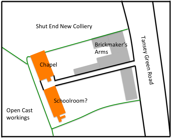
The 1859 redrawing of the Pensnett portion of the 1840 map shows no change to the chapel but there were by then mines to the north of the plot and open cast workings to the west. By the 1883 OS map (figure 2) the Schoolroom was present, and the open cast mine to the west was very clear. Both the Chapel and the Schoolroom were rectangular in form, roughly 14m by 8m in plan. After the congregation moved to the new building on Commonside (the Independent Methodist Chapel, it would seem that the buildings were in use as a sewing factory. The 1910 map indicates that they had become a “Picture House” and the Chapel and Schoolroom had been joined together into one long structure.

**Figure 2. The chapel and schoolroom (from the 1883 Ordnance Survey map)**

No details of the interior of the building survive, but these can perhaps be conjectured by what was built to replace them on Commonside. This had a balcony at the front of the chapel for the choir and organ, with the raised preaching desk and the table for the Lord’s Supper placed centrally at the front of the Chapel beneath the balcony. Pews occupied the rest of the chapel building. Although the original chapel was unlikely to have had a balcony, it would almost certainly have had a preaching desk / pulpit of some sort of simple communion table at the north end (probably beneath where 6a Renown Close now is.

As noted in the Introduction above in the 1850s there were three services on a Sunday – morning, afternoon and evening. In the latter years of its life various directories in the 1880s indicate that there were only two services on a Sunday – at 10.45am and 6.00pm, but there was also a mid week service on Wednesday at 7.30pm, which probably existed throughout the life of the chapel. Similar midweek services were common practice for all the churches in the area at that time. The dates in the baptism register indicate that baptisms could occur on Sundays and also on other days.

In the second post of this series, I will begin my consideration of the Baptismal Register from 1845 to 1887, and in particular look to see what this document says about the overall nature of the congregation – where thy lived, the jobs they did, and the names they chose for themselves.

Caring for God’s creation (V)

A presentation is from the very early days of lockdown – a recording of material I was meant to present at a Lent course on environmental issues that never actually happened.

Vehicle restrictions during windy conditions on long span bridges

The Bridges

Around the UK, there area number of relatively long and high bridges across river estuaries, that all operate some sort of traffic restriction protocol in high wind conditions, to limit the risk of vehicle accidents. In this post, I will attempt to collate publically available information on these traffic restriction protocols to assess their similarities and differences. It will be seen (surprisingly in my view) that this information is not at all easy to find and sometimes does not seem to be in the public domain. .

The bridges that will be considered are shown in Table 1, which gives name, location, construction type and length. Pictures of them are given in figure 1. It can be seen that, with the exceptions of the Cleddau Bridge in South Wales and the Skye Bridge in Scotland, these are all over a kilometer long. The construction types vary, from concrete boxes on large numbers of concrete piers to long span suspension and cable stay structures. Only two bridges in the table have protection for vehicles against cross winds – the Prince of Wales (Second Severn) Bridge and the Queensferry Bridge in Edinburgh. All the bridges in the table have Wikipedia entries, which give further details of planning, construction and operation.

Vehicle restrictions

The data for wind speed restrictions was found from a variety of sources – official documents, FOI releases, newspapers etc. The information that has been obtained is shown in Table 2. Most have a similar form, with different levels of restriction being used as the gust wind speed increases – vehicle speed limits, lane closures, restrictions to various classes of vehicles, and total closure. Most seem to base the wind speed values on local anemometers, although it is usually not clear where these are sited, and neither is the period of the gust given. Thus the values that are given are not strictly comparable with each other in absolute terms.

**Table 2 Wind speed restrictions**
(H- Headwind, C – Crosswind, * values are given in mph in table, but equivalent values in knots are used in practice)

From table 2 it can be seen that no data could be obtained for the Kessock Bridge, the Humber Bridge or the Prince of Wales (Second Severn) Bridge. With regard to the latter, vehicles crossing the bridge are shielded by wind fences and the bridge has not had to impose restrictions on traffic during its lifetime. Kessock probably has the same sort of traffic restriction strategy as the other Scottish bridges, as Transport Scotland operates a common approach. From press reports it seems that Humber has some sort of vehicle speed limit and high-sided vehicle restriction strategy, although it has not been possible to determine the wind speeds at which the different measures are put into place. . Also note that Queensferry has much higher values of wind speed for restrictions than the other bridges, again due to the fact that vehicles are protected by wind fences.

For the other bridges, there seems to be a general consistency in the information shown, with vehicle speed limits of either 30mph or 40mph imposed when the wind gusts over 35 to 50mph. Vehicle restrictions begin at gusts of around 45mph to 60mph, with double deck buses and high sided vehicles being restricted at the lower gust speeds. Further restrictions may be imposed on vehicles of different types, before overall bridge closure at wind speeds of 65 to 80mph. Some bridges use different gust speeds for cross winds and for headwinds. Orwell Bridge for example applies the crosswind criterion if the wind gust direction is from a sixty degree segment centred on the direction normal to the bridge. The Queen Elizabeth II Bridge at Dartford uses similar strategies to inform speed limits, lane closures, vehicle restrictions and bridge closure.

The restriction strategies depend very much on the nature of the traffic over the bridge and its location. For example, if only some vehicles are to be restricted, then some method of filtering them out and diverting them is required, which needs to take place at some distance from the bridge. Such procedures are in operation at Severn, Erskine, Humber and the Queen Elizabeth Bridges amongst others. Clearly ease of identification of vulnerable vehicles is required – see figure 2 for the Humber Bridge. Other bridges simply base their protocols on vehicle height eg 1.9m for Cleddau and 2.1m for Severn.

Description: Macintosh HD:Users:chrisbaker:Dropbox:Web site:Blog material:Crosswinds:Bridge closure:Humber.png — **Figure 2 Humber Bridge High sided Definition**

Orwell Bridge operates a very simple strategy, with different gust speed triggers for crosswinds and headwinds, leading to complete closure, without any restrictions for, say, high sided vehicles at lower wind speeds. This arises because of the urban nature of its surroundings, which makes vehicle filtering difficult. This has led to a considerable number of closures in recent years, and much public concern. Recently both numerical and wind tunnel studies have been carried out to investigate ways in which this strategy can be modified, perhaps through the use of speed limits, lane restrictions or barriers. The details of these studies have not been released to date but may prove of some interest. Studies to relax the restrictions on Skye Bridge have also been recently carried out following frequent closures and public complaints.

As can be seen, the various restriction strategies are in general quite simple and easy to operate. This inevitably means that they are conservative and largely based on the most vulnerable vehicle – usually unladen high sided vehicles. There are in fact methods available for discriminating between vehicle types and vehicle weights – see the recent paper by Baker and Soper (2019) for example. This gives a method for determining a curve of accident wind speed against vehicle speed for specific vehicle type and weight, based on which restrictions strategies for any particular vehicle can be determined. However operational constraints make the full utilisation of such methods difficult. Until such time as vehicle type and vehicle weight can be automatically determined by (say) remote visualisation techniques and dynamic weight determination, and vulnerable vehicles can be suitably diverted, then the use of simple methods such as those currently adopted will remain the best that can be achieved.

Specifying accident windspeed risk

This post is intended to start a discussion – and ideally identify what data might be available to address this problem further. The analysis presented is preliminary in nature, and could almost certainly be refined. I would really value a discussion of this with colleagues who read it.

Accident risk

In studies of road and rail vehicles in cross winds, some estimate of the risk of an accident is often required. If the critical accident wind speed for a particular vehicle is known, then my approach in the past has been to use the probability distribution for the hourly mean wind speed (assumed to be a Weibull distribution) and the probability distribution for the turbulence fluctuations around this average (assumed to be a normal distribution) to calculate the percentage of time that this critical value is exceeded, through a convolution of the two distributions. Additionally, when wind-warning systems are being developed, the question often arises as to what would be an appropriate mean wind speed at which to limit vehicle movements. This can be derived by calculating the percentage of time that the critical wind speed is exceeded from the probability distributions for turbulence fluctuations, for a range of mean wind speeds, and then choosing a value that has an acceptable level of risk.

In some recent work that I have carried out for a particular client, it has become clear to me that this approach is not really adequate – an example of practical reality not always conforming with attractive theoretical approaches! Both road and rail vehicles require a gust to be above the critical value for a specific period of timebefore an accident occurs. This period of time is usually between 0.5s and 3s, the time it takes for a vehicle to actually blow over. Thus in determining the risk of an accident what is really required is some idea of the number of times the critical wind speed is exceeded, N, for more than (say) T seconds for a particular mean wind speed U. This is not the same as the proportion of time for which the critical wind speed is exceeded, as some these exceedances will often last for less than T seconds. If the probability of N for any particular U is known, then this can be convoluted with the probability distribution for U to calculate the overall risk, or used to determine an appropriate value of U for wind warning systems.

To the best of my knowledge, the specification of the number of gusts N lasting greater than a specific time T for a particular mean wind speed has not been investigated in the past – but if any reader knows of such work, I would be glad to hear of it. In this post, I present the results of a preliminary investigation into this problem.

The data

In what follows, I will use two experimental wind datasets as follows.

Data from that late 1990s obtained at the Wind Engineering field site at Silsoe Research Institute, and in particular two one-hour datasets (Silsoe 1 and Silsoe 2) with wind velocities measured at 10Hz at 3, 6 and 10m above the ground, for 10m wind speeds of 9.7 and 10.5m/s.
Data from Storm Ophelia in 2017, obtained from measurements at the top of the Muirhead Tower at the University of Birmingham, 72m above the ground, measured at 10Hz, for mean hourly wind speeds of 10.4, 12.5 and 13.8m/s (Birmingham 1, Birmingham 2 and Birmingham 3). With thanks to Dr Mike Jesson of the University of Birmingham for making this data available

The basic statistics for each hour of data is given in table 1.

From this table it can be seen that the Silsoe site has a surface roughness length (determined from velocity profiles) typical of smooth rural environments (0.005m), with turbulence intensities (standard deviation / mean values) that are consistent with such an environment and which fall slightly with height. The Birmingham data was obtained at one point high above a suburban environments, and thus the surface roughness length cannot be determined from a velocity profile, but can be expected to be an order of magnitude or more higher than at the Silsoe site. The turbulence intensity is similar to that measured at Silsoe, although the measurements were made at a much greater height above the ground. For the Silsoe data the probability distributions of the data all show a positive skew, whilst the Birmingham data show both positive and negative skew values that are much closer to zero. Typical examples of such distributions are shown in figure 1. The Silsoe near-ground distribution has a significantly longer upper tail, than the Birmingham values high above the ground, i.e. a significant skew towards the higher velocities. This may well be because of individual sweep events in the atmospheric boundary layer being more significant near to ground level. The normal distribution, which I have assumed in the past for my calculations, does not fit either dataset particularly well.

**Figure 1 Wind Probability distribution**

Analysis of exceedances

The approach to using this data has been to find, for each dataset, the number of exceedances N for T= 0.5s, 1s and 3s gusts above a range of velocity levels above the mean. To enable comparison between the different datasets, these velocities are expressed in terms of standard deviations above the mean, denoted by X. The results are shown in figure 2 for the Silsoe data and figure 3 for the University of Birmingham data. The following comments can be made.

N falls as T increases, which is only to be expected.
The value of X at which N falls to zero falls as T increases, as again is to be expected. This value is around 3 to 3.5 for the Silsoe data, and 2.5 to 3 for the Birmingham data, reflecting the form of the tail of the probability distributions discussed above.
For the Silsoe data, the results for the two datasets are very similar and there is an indication that N varies with height above the ground.
The Birmingham datasets also have similar results, and there is no discernable effect of wind speed in the data when plotted in this way.

**Figure 2 Number of exceedances (Silsoe data)**

**Figure 3 Number of exceedances (Birmingham data)**

Clearly the distributions of N have an upper limit. This can be characterized in two ways.

By the value of X for which the probability of the wind speed exceed T/3600, X₁
By the highest value of X for which N>0, X₂

Both these values of X are shown in table 2 for the various datasets. It can be seen that there is some variability in the results, which is inevitable as we are dealing with the tails of the distribution where data becomes discontinuous. In general the values for X₁are higher than those for X₂, particularly for the near ground Silsoe data, suggesting that the use of simple probabilities rather than gust numbers may well significantly overestimate vehicle overturning risk. Both values fall as the time period T increases as would be expected, and the values for the Silsoe data are significantly higher than for the Birmingham data, which again follows from the difference in probability distributions. The equivalent values for X₁ for a normal probability distribution are 3.64, 3.45 and 3.14, for T= 0.5, 1 and 3s respectively. It can thus be seen from Table 2 that the Silsoe values lie above the normal distribution values, and the Birmingham values lie significantly below them.

The data from figures 2 and 3 thus appears to be consistent and sensible, but the question then arises as to how this data can be parameterized to enable it to be used easily in calculations. After some trial and error analysis it was found that all the data for each site could be made to collapse around a single curve by plotting the combined variables NT and (X₁-X)/X₁ against each other. These variables seem sensible, as both are dimensionless, with the former giving a normalised value of number of exceedances, and the latter describing being the difference between specific gust velocities, and the value at which N must be zero. The results are shown in figures 4 and 5 for the Silsoe and Birmingham data respectively, using the measured values of X₁ for each dataset. It can be seen there is much scatter, but the data collapse is reasonably good. The two sets of data do not however coincide, indicating the effects of the underlying shape of the probability distribution, and in particular the upper tails.

**Figure 4. Analysis of Silsoe exceedance data**

**Figure 5. Analysis of Birmingham exceedance data**

The region of most practical interest on these data collation is for a low number of events, since these represent conditions where the risk might be tolerable. Thus figures 6 and 7 thus show expanded versions of figures 4 and 5 for NT<50. It would quite possible to fit lines or curves to this data, although the best fit values would be different between the Birmingham and Silsoe datasets.

**Figure 6. Expansion of figure 4 for low NT values**

**Figure 7. Expansion of figure 5 for low NT values**

It would seem that if this method is to become useful in a predictive, rather more detailed information on near ground probability distributions is required for a variety of ground roughness conditions / heights above the ground etc., so that the variation in the exceedance curves of figures 4 to 7 can be more fully understood and an overall data collation be achieved. If any reader knows of systematic data for wind probability distributions, please let me know.